Conjugate Heat Transfer Analysis on a graphics card.

Aim:

Conjugate heat transfer Analysis on Graphic Card.

Objectives:

1. Run the simulation by varying the velocity from 1m/sec to 5m/sec for at least 3 velocities and discuss the results.
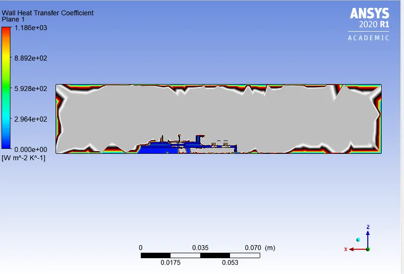
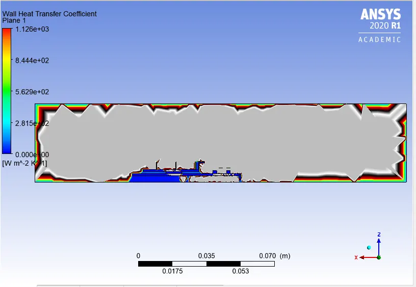
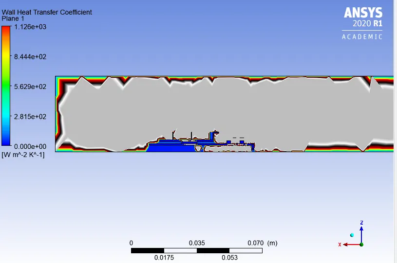
2. Find out the maximum temperature and heat transfer coefficient attained by the processor.
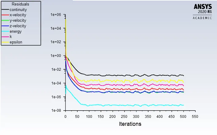
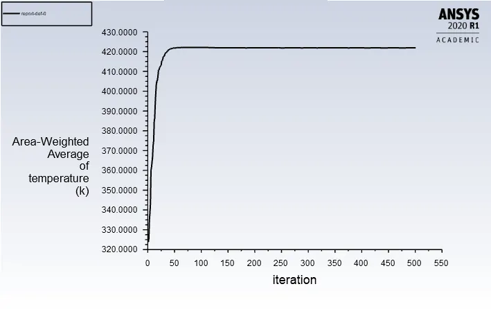
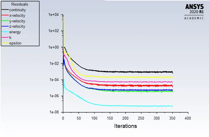
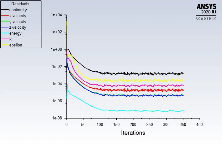
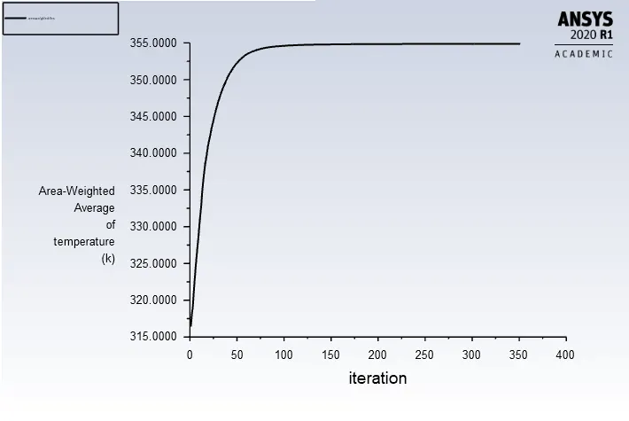
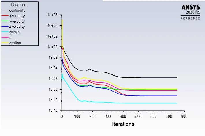
3. Prove that the simulation has achieved convergence with appropriate images and plots.
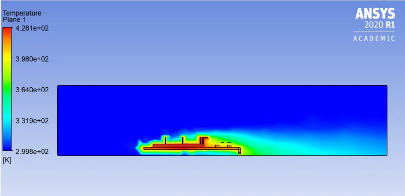
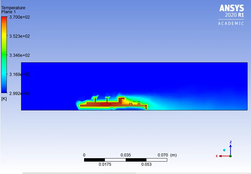
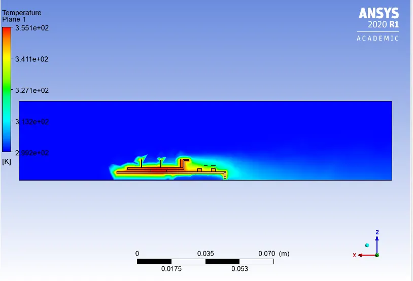
4. Identify potential hotspots on the model.

Introduction:

CHT refers to the heat transfer from inside the solid boy to the outer surface and thus from the outer surface to further dissipawattson of heat via convection. Thus a realisitic approach of this for this analysis is required to understand the heat disspation and the heat transfer rate along the two different bodies. This task is generally accomplished with the continuity equation and the heat flux transfer at the interfaces as teh governing equation.

In our case the graphic card has three main components,

1. The PCB base, which consists of the micro circuitries and the set of capacitors and resistances which make the complete cuircuit.
2. The processor, the brain of the graphic card which is responsible for all the work and tasks being carrird out thus a processor in a graphic card generates the maximum amount of heat and will be used as the source term in our project.
3. The fins are the mechanical device which has a lot of pins coming out from it to increase the surface area thus increasing the amount of the heat disspation in the processor.

Generally a cooling fan is prvded in the PC's for the heat disspation of the graphic card to induce the forced convection as the fins nd natural convection itself are not ssuffiecient for the mount of heat generated. Thus to simulate the cooling effect in the fan we will be working with the inlet velocities and we will range it from various magnitudes to check the effectiveness of speen on the graphic card.

Assumption:

1. The prcessor is the only heat source in our analysis, Generally the memory RAM and other devies also generate heat but to simplfy our problem we will only use processor as the heat source.
2. Power consumed by the processor 9.6watts
3. The heat generated by the processor=9.6/10^-9=15*10^7W/m^3. (This is the maximum heat that can be generated by the processor if all of its energy is convereted into the heat energy without any loss).

Methodology:

1. Modeling the graphic Card
2. Meshing
3. Pre-Processing
4. Setting up Physics
5. Post- Processing

Modeling

The model of the graphic card can be generated by using any of the CAD softwares which can then be convereted into the .stp, .igs or .x_t file. This file can then be imported in the ANSYS Spaceclaim Model as shown below:

When the geometry in imported it can be repaired if any extra edges or any error is found then an eclosure is made around the body for teh simulation and then the geometry is shared between the enclosure and the Graphic card. This is done such that the data such as physical properties can be shared from the encolure with the graphic card.

Meshing:

Meshing the grid and the grid size plays an important role and the limitation of the educational licesnce also plays in vita role in the mesh size because it couldnt make a grid size too fine and there is also limit on the number of fces in the educational license. Further a mesh size shuldnt be made too fine without proper explaination because solving such a fine grid size will take a lot of computational recources and also degrades the mesh quality which brings a lot of errors while solving and too course mesh size dont predict the flow parameters accurately. Thus nitially for the first run we will proceed with the baseline mesh and see thus after checking the result we will define the areas where refining is required. Apart from mesh we will also prvide the names to the boundaries thus helping us to provide the bounday conditions as shown below:

Preprocessing:

After successfully making teh mesh we will start with the setting up the physics. We will first check for any errors in the meshand give the definations as

Simulation Type: Steady State

Solver: Pressure Based

Turbulence Model: Realisable K-epsilon Turbulence model will be used because we are intersted in flow of fluid and the heat disspation rather than what is happening near the boundaries of the graphic card.

The energy equation will be turned on to study the transfer of the heat from the body to air.

Further we will add materials accordingly in our database from the fluent database. For our model we have made the

Base-Copper(Generally teh base is made of composite consisting of copper silicon and other materials which can be made manually in the fluent database, But for simplicity we will use copper)

Processor-Gold (Processor is also made with the composite of gold silicon and different materials but again for simplicity we will be using gold).

Fins- Aluminium

Now we will define the cell zones and assign the properties (solid and fluid) and materials to the different bodiesand the enclosure as the air. Also we will provide the heat source to the processor as the 15*10^7W/m^3.

We will provide the initial inlet velocity with 1m/s for the first baseline mesh inlet temperature will be 300K.

The outlet will be set as the pressure outlet with the 0gauge pressure. Rest all the wall boudries will be left with the coupled boundary condition. The solution will then be initialised with the hybrid initialisation and will be set with the 350 iterations.

The results can be seen below:

1.Residual Plot

2. Area Weighted Temperature

3.Temperature Plot on the Mid Plane

4. Wall heat transfer Coefficent on plane

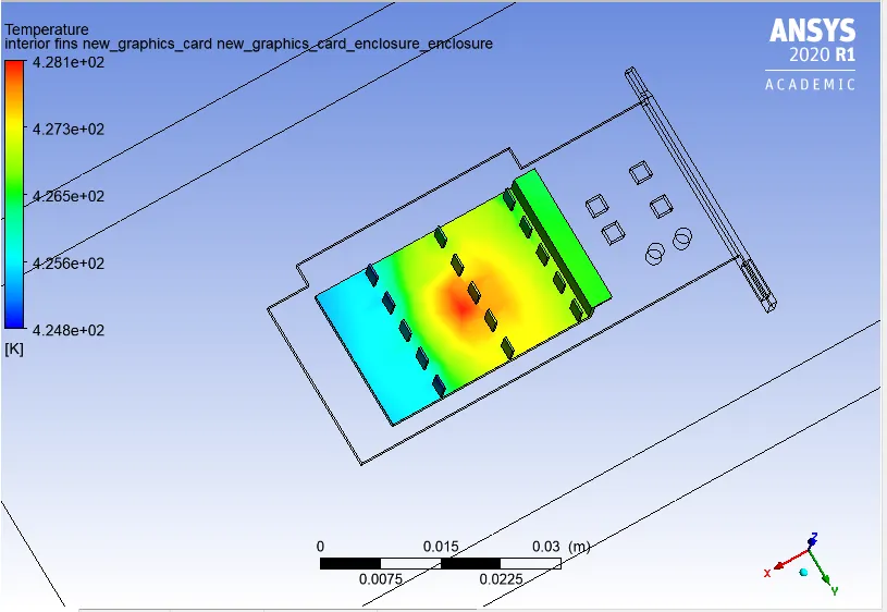
5.Hotspot Region (Fins)

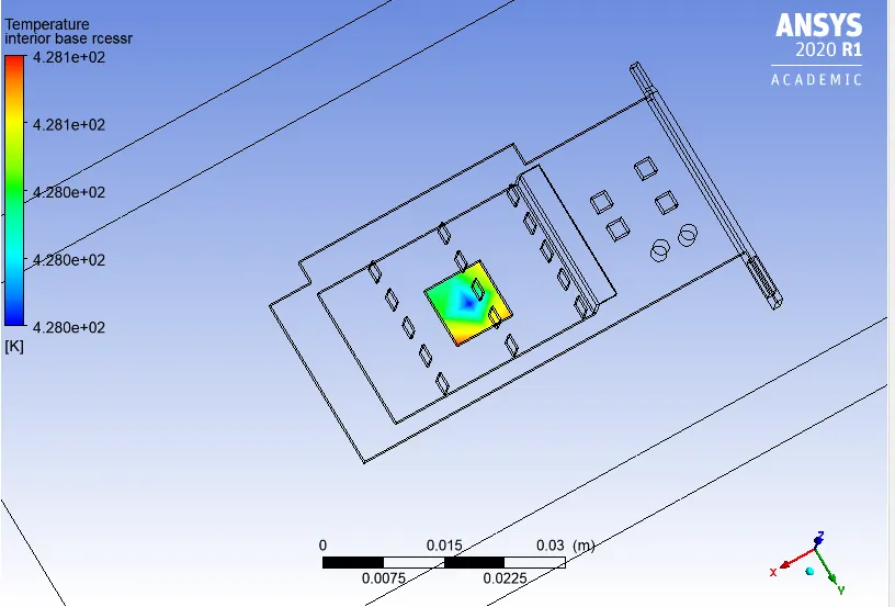
6.Hotspot Region (Processor)

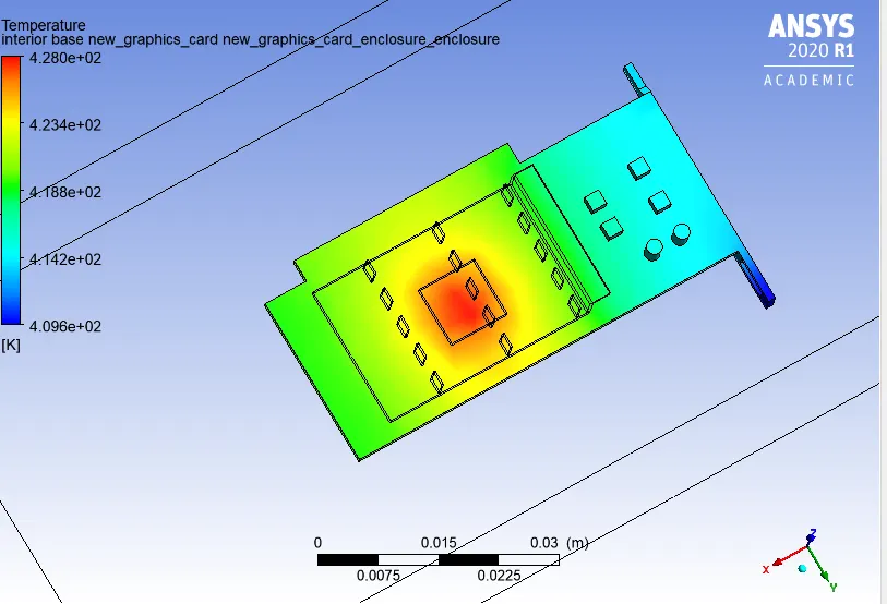
7. Hotspot Base (PCB)

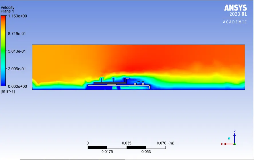
8. Velocity Mid Plane

Futher the base line mesh will be run again for this analysis for the inlet velocity of 3m/s and rest of the parameters will be same.

The results can be seen below:

1.Residual Plot

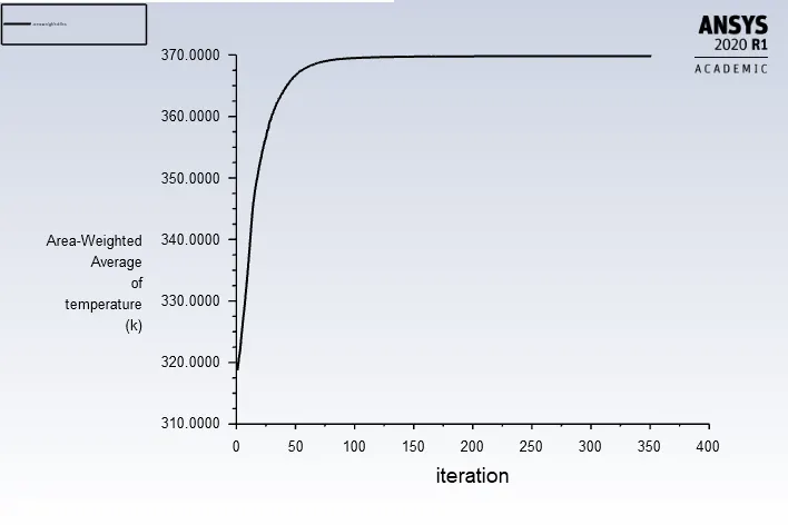
2. Area Weighted Temperature

3.Temperature Plot on the Mid Plane

4. Wall heat transfer Coefficent on plane

5.Hotspot Region (Fins)

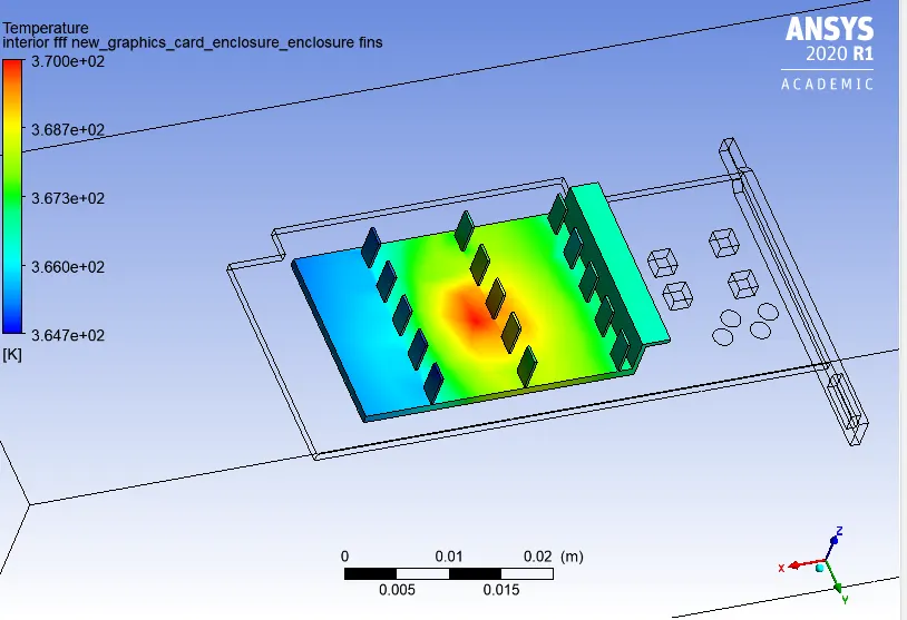
6.Hotspot Region (Processor)

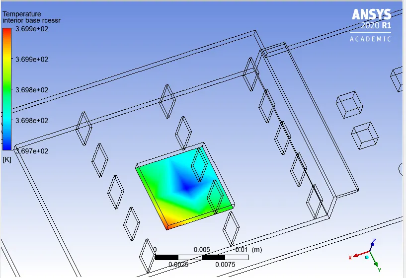
7. Hotspot Base (PCB)

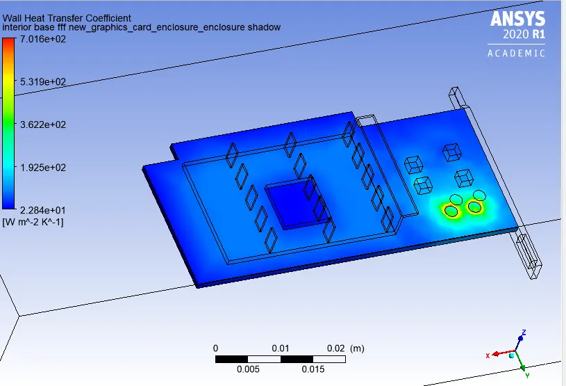
8. Velocity Mid Plane

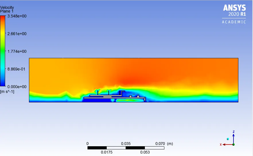
Futher the base line mesh will be run again for this analysis for the inlet velocity of 5m/s and rest of the parameters will be same.

The results can be seen below:

1.Residual Plot

2. Area Weighted Temperature

3.Temperature Plot on the Mid Plane

4. Wall heat transfer Coefficent on plane

5.Hotspot Region (Fins)

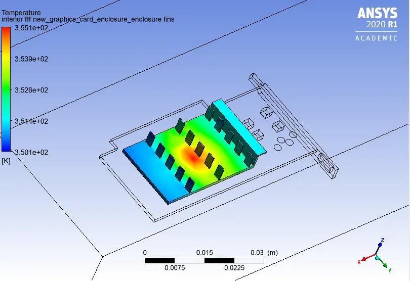
6.Hotspot Region (Processor)

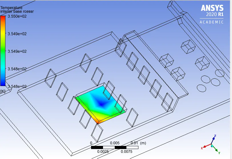
7. Hotspot Base (PCB)

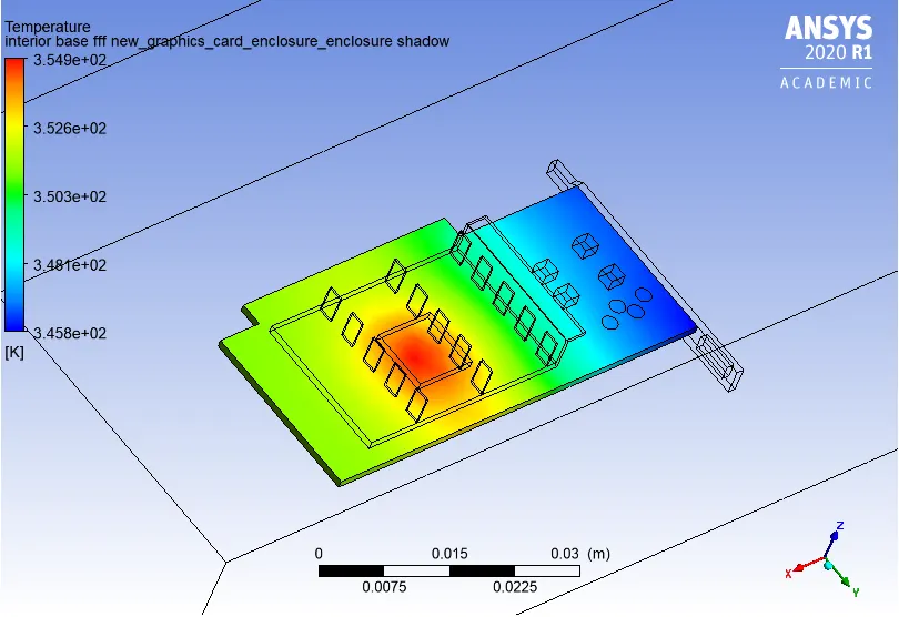
8. Velocity Mid Plane

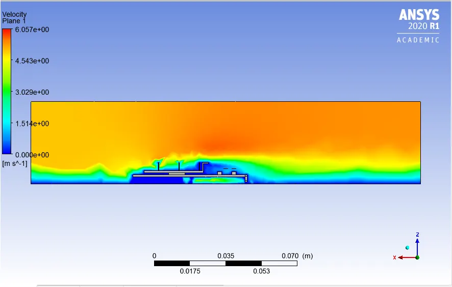
Case II Refined Mesh

In this case we will be refining the mesh by using the body sizing for the different components. As in educational license we cant beyong 0.5 million cells thus element size is set as shown below:'

1. Body Sizing Base- 0.75mm
2. Body Sizing fins-0.5mm
3. Body Sizing Processor- 1mm
4. Global Body Sizing-3.5mm

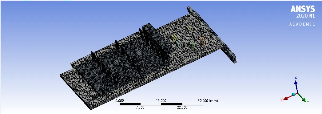
The mesh can be seen below:

The Named Selections can be seen below:

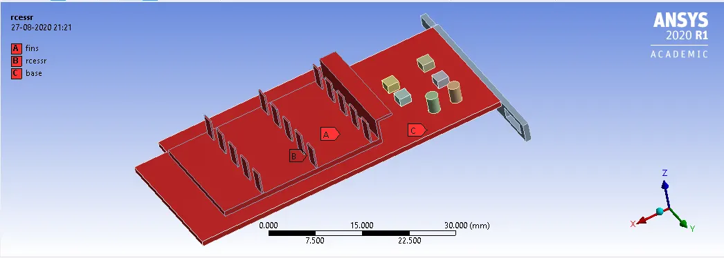
The Total Number of nodes are 83642 and the number of elements are 479668. The Mesh Quality can be seeen below:

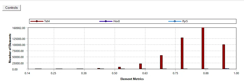
Here it can be seen that the mesh quality is minimum of 0.14 percent which is above 0.1% and maximum mesh quality 88% thus the overall meshing for this element can be considered good and is within the range of 0.5 million cells of educational lisence.

Preprocessing

The mesh will be checked first and the simulation boudary conditions will be given as in the first case and the simulation will be run for more iterations as the convergence will take time due to large number of cells.

The simulation willl be done again for three input velocities as 1m/s, 3m/s, 5m/s.

The results for 1m/s can be seen below:

1.Residual Plot

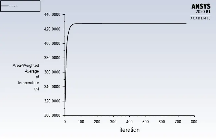
2. Area Weighted Temperature

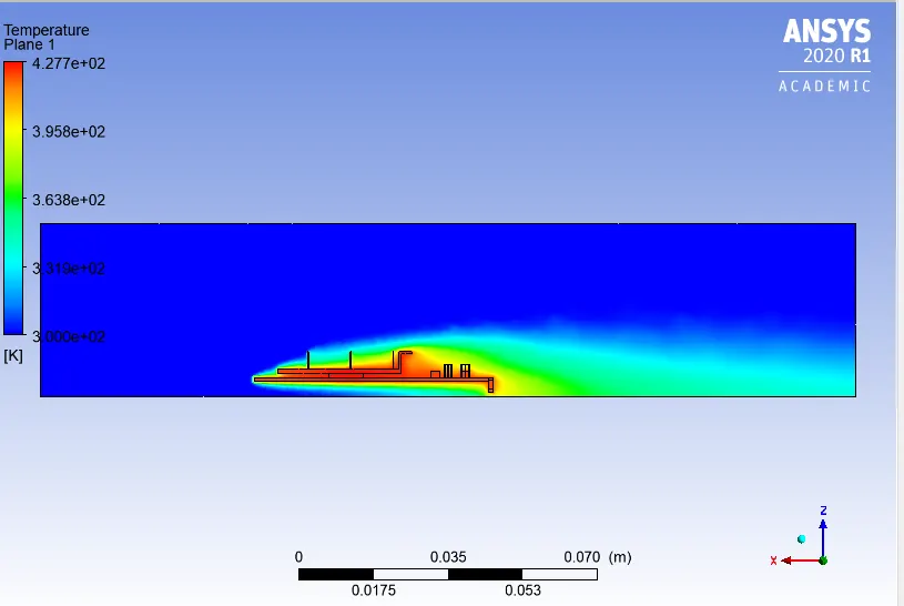
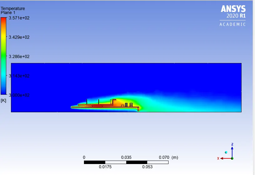
3.Temperature Plot on the Mid Plane

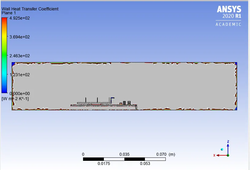
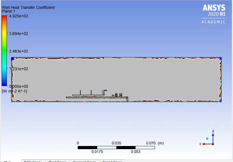
4. Wall heat transfer Coefficent on plane

5.Hotspot Region (Fins)

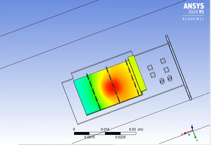
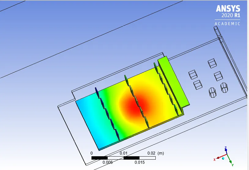
6.Hotspot Region (Processor)

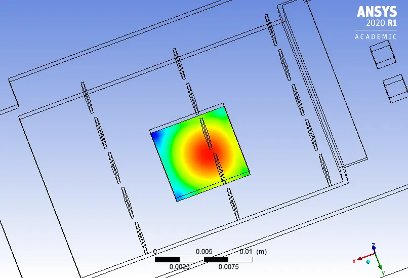
7. Hotspot Base (PCB)

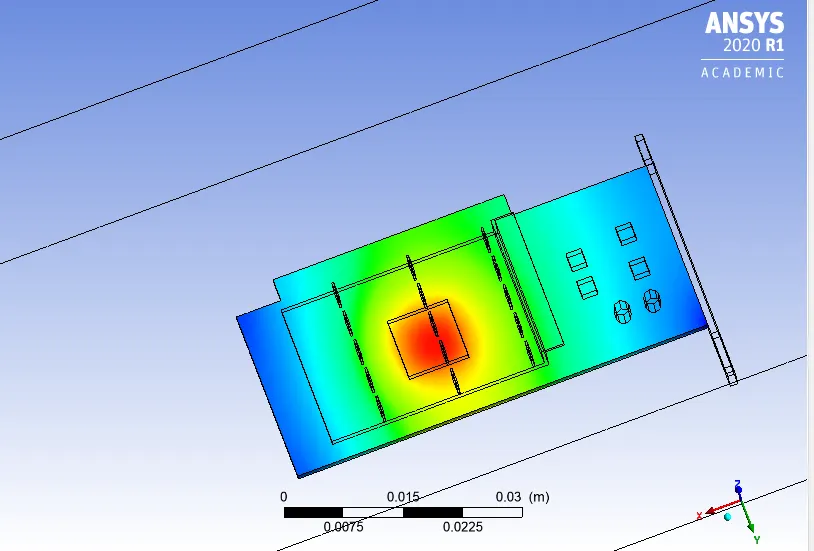
8. Velocity Mid Plane

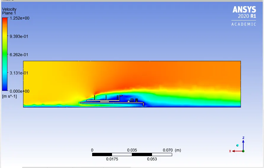
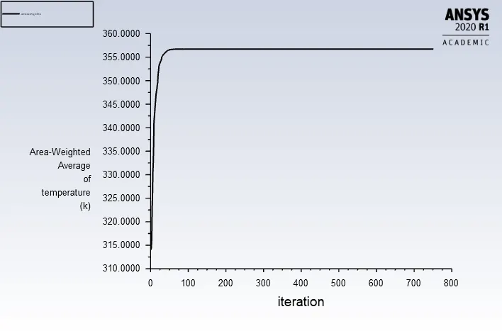
The results for 3m/s can be seen below:

1.Residual Plot

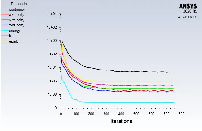
2. Area Weighted Temperature

3.Temperature Plot on the Mid Plane

4. Wall heat transfer Coefficent on plane

5.Hotspot Region (Fins)

6.Hotspot Region (Processor)

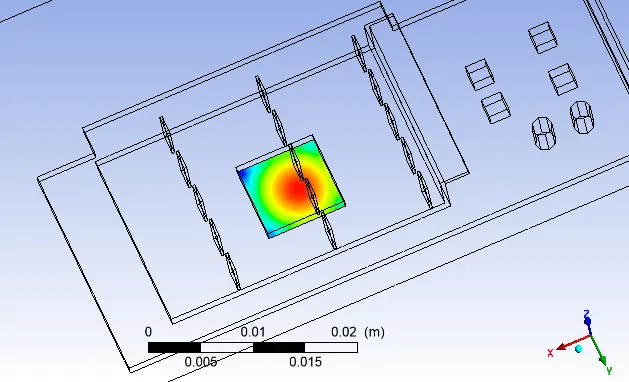
7. Hotspot Base (PCB)

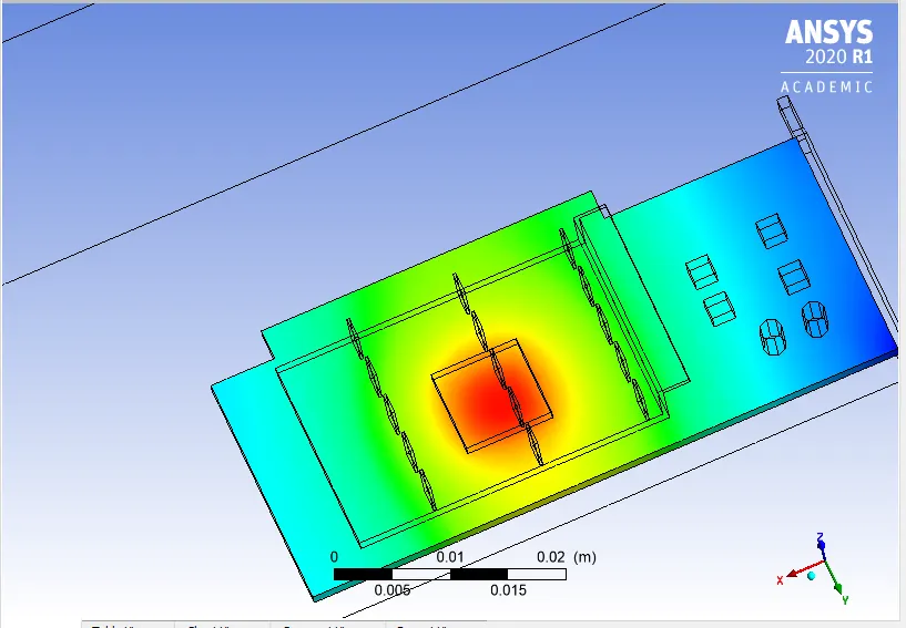
8. Velocity Mid Plane

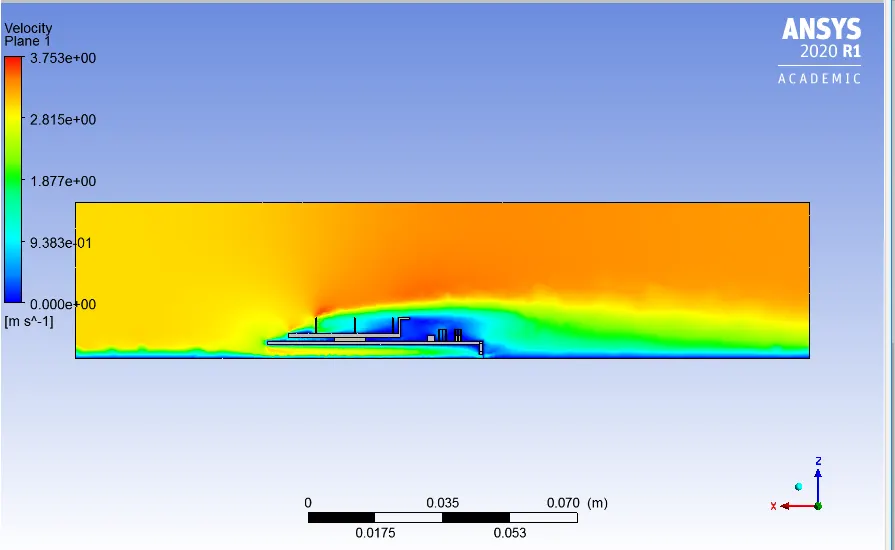
The results for 5m/s can be seen below:

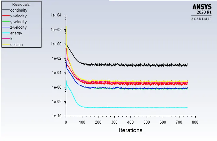
1.Residual Plot

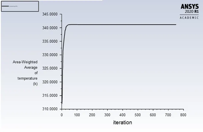
2. Area Weighted Temperature

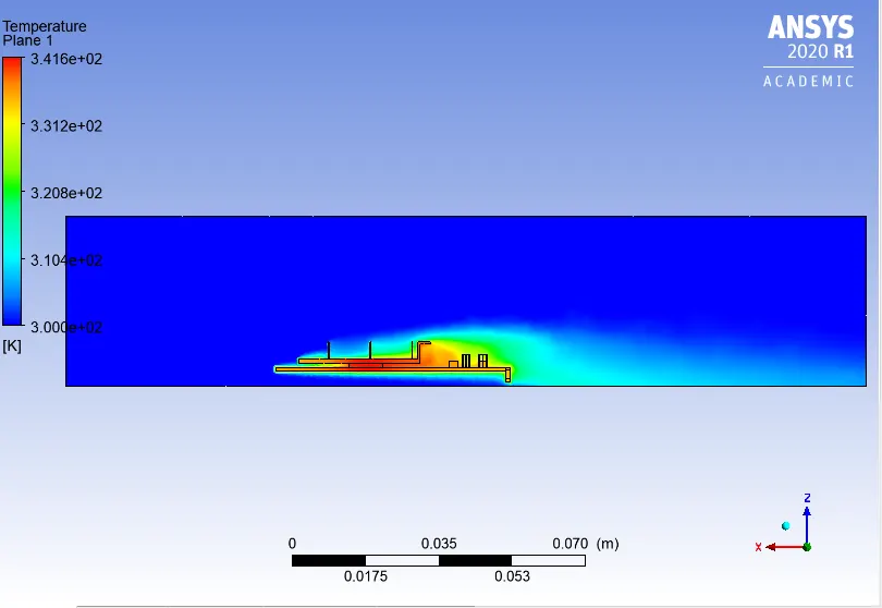
3.Temperature Plot on the Mid Plane

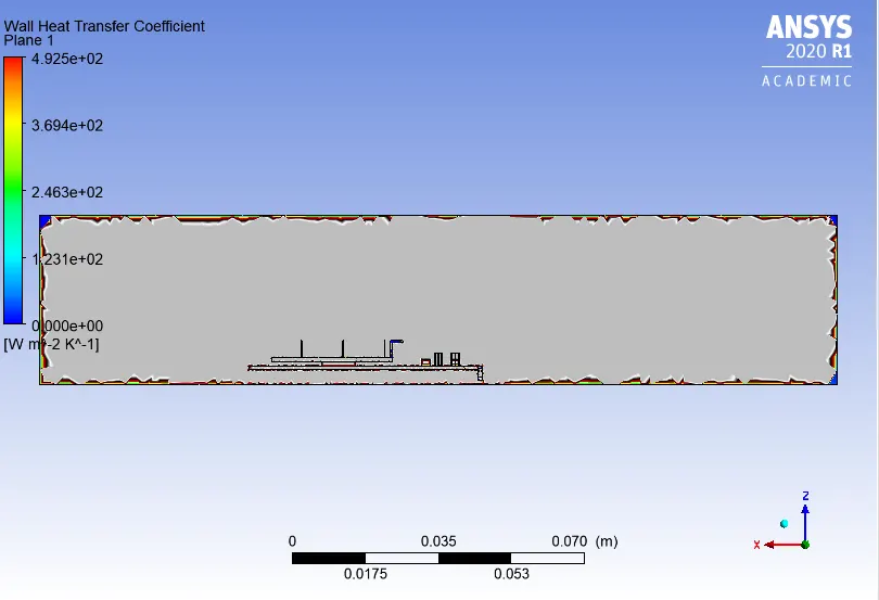
4. Wall heat transfer Coefficent on plane

5.Hotspot Region (Fins)

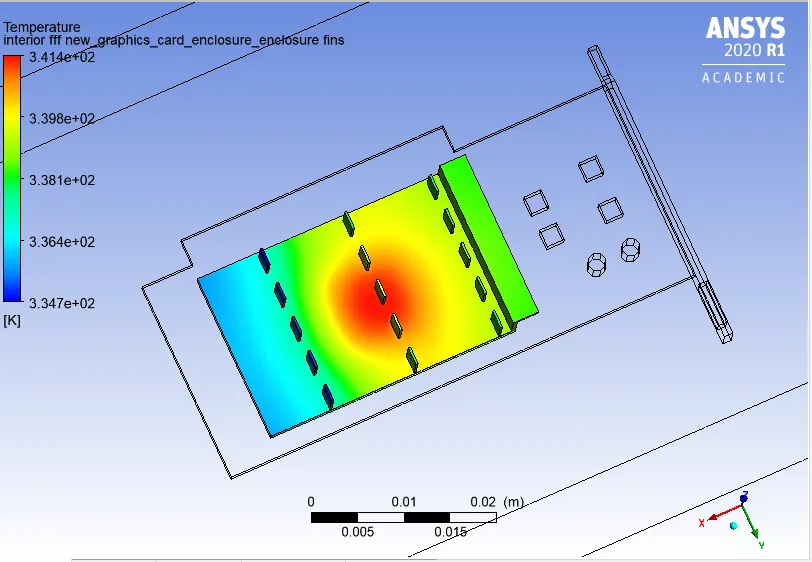
6.Hotspot Region (Processor)

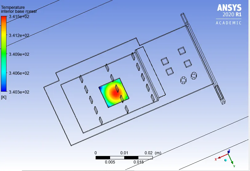
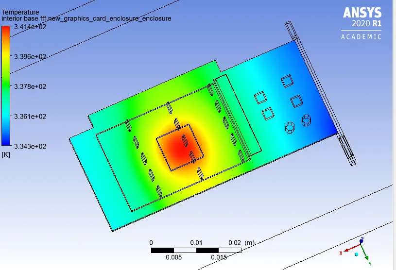
7. Hotspot Base (PCB)

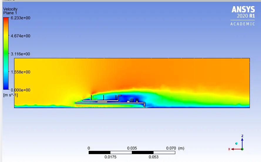
8. Velocity Mid Plane

Results and Observations:

The result from the above simulation can be seen below in table:

	Baseline Mesh	Baseline Mesh	Baseline Mesh	Refined Mesh	Refined Mesh	Refined Mesh
Velocity	1	3	5	1	3	5
Max Total Temp.	428	370	355	430	357	341
Temperature Area Weighted Average	420	370	355	427.7	357	341
Max. Heat Tranfer Coeffficient	1186	1126	1126	4925	4925	4925
Base Temp Hotspot	428	370	349.9	427.5	356.97	341
Processor Temp Hotspot	428	369.9	355	427.67	357	341
Fins Temp Hotspot	428	701.6	355	427.67	357.138	341

Here we ran the simulation for the above shown results and got the converged results as shown in the residual plot for each individual solution.

Here, we started with the baseline mesh and then after refing the results we can see that we approached a more exact solution. Thus from the above results it can se said that the baseline mesh are not good for cap[turing the exact solution and the tumperature distribution at the interfaces.

Fins were given in the GPU to increase the heat transfer coefficient rate for the processor. As the processor is only heat source in the GPU th eFin is directly joined to it reduce the heat generated . Furyher when the velocity is increased from 1m/s to 5m/sit is also seen that the heat dissipation process also increases as it induces more convection thus increases heat transfer coefficient thus decreasing the max temperature in the enclosure.

Conclusions

1. Heat transfer rate is directly propotional to inlet velocity.
2. Mesh plays an important role in finding the exact solution and also the heat transfer coefficient.
3. Fins are used in the these assembly because they increase the surface area of the source body thus increasing the heat transfer and interaction between the interface.
4. Inflation Layers are not used generally for these types of complex assembly because they degrade the mesh quality thus initialting the errors in the assembly.