Conjugate Heat Transfer Analysis on a graphics card.
Computational Fluid Dynamics Simulation on Heat Sink Performance by Varying Inlet Velocity
Abstract
The study on heat transfer has attracted the attention of many researchers because of its significant impact in ncreacing the efficiency of engineering and industrial application. One of the applications is a heat sink performance of a graphics precessing unit (GPU) thermal management and impact of it on the thermal performance. So what's actually happening is that GPUs in high-performing graphic computing become heat source. As temperature increases, the performance of the graphics card drops causing the same to graphic performance and extreme case, causing the computer operation to stop. Some measure have to be taken for that, there comes the Heat Sink . Heat sink basically increases the exposed surface are and via conduction heat is liberated across the heat sink and via Forced convection heat is propogated to the cool air(relative to the processor environment) that is comming from the inlet.
But its very difficult to see what's happening there inside the CPU case, so whe depend upon the CFD simulation to investigate and observe the heat transfer of heat flow inside a computer case and heat sink in order to solve the overheating issue.
Methodology
A simplified Graphics card is modeled to represent a real GPU that is available in the market. GPU contains Fins (heat sink) , Processor and Base. Along with the GPU a wind tunnel is modeled with inlet and outlet, where the airfolw is occuring. A monitoring Plane is constructed along Y-Z plane where the folw contour is obsereved.
To simulate all these phenomenon, Ansys Fluent is used. Fluent is a computational code that allow the user to solve the physics and substantially reduces the expensive remote machine.
Geometry Configuration
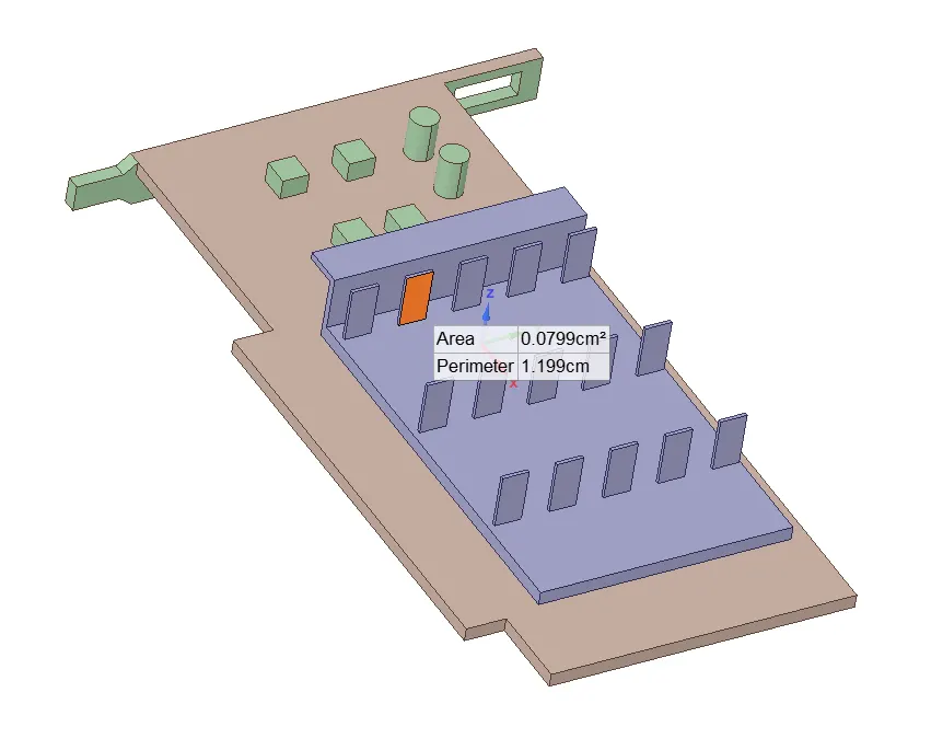
Fig1 This is the 3D geometry of GPU with fins area indicated
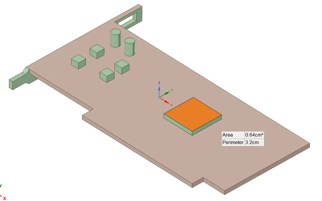
Fig2. This is the base with processor attached with area indicated above
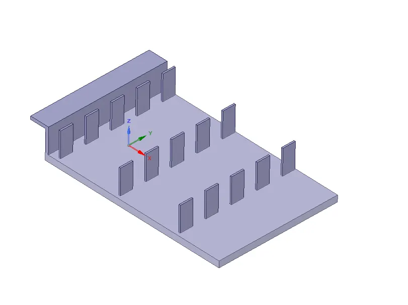
Fig3. The above fig is fins that is the main component for reducing temperature
- Area of the Fin- 0.0799 `cm^2`
- Area of the processor- 0.64 `cm^2`
- volume of the processor- 0.064 `m^3`
Boundary Condition
The air flow consist of air inlet and pressure outlet which which have wind velocity of 1 m/s , 3 m/s and 5 m/s. These three different velocity condition are three cases that is being simulated and studied in this project.
The air is assumed as steady flow and incompressible throughout the flow, and the air density is constant, 1.225`(kg)/(m^3`.
The temperature of the air is assumed to be same as the room temperature 300 k.
The pressure of the air is assumed as ideal atmospheric pressure, 101325 Pa.The type of air flow is modeled as asegregated flow which is suited for incompressible flow. The air is modeled as turbulent as the Reynolds number achieves Turbulent criteria for internal flow (Re > 4000). So, air is modeled into Reynolds-averaged Navier-Stokes because this is an equation for time-averaged equation of motion for fluid flow and primarily used while dealing with turbulent flow.
And for that `k-epsi`turbulent model is selected as it is most common model to simulate mean flow characteristic for turbulent flow.
Regarding the Graphics card, the time is modeled as Steady as the heat released by the processor chip is constant flow at any point. Base, fins and processor are modeled as solid with an initial boundary condition of Wall temperature of 300 k. At a wall boundary, we may specify either (i) the wall temperature or (b) the wall heat flux, but not both, as this would be mathematically over-specified.
The processor heats up when it's involved in high computing so act as a heat source so it was modeled as a heat source.
Calculation of heat flux-
I considered it as my laptop GPU which is Nvidia GTX 1650 Ti, which uses power of 83 W [1], in normal computation.
So Wall heat flux= (power uses)/(volume of processor aka heat source)= `(83*10^6)/0.064 W/m^3= 1,29,68,75,000 W/m^3`.
| Component | Material |
| Heat source | Aluminium |
| Base | Copper |
| Fins | Aluminium |
Table 1. Material for each component
Mathematical Modelling
Governing Equations
It is often called the equation of continuity because it requires no assumptions except that the density and velocity are continnum functions. That is, the Flow may be either steady or unsteady, Viscous or Frictionless, Compressible or incompressible. The equation of continuity is:
`(delrho)/(delt)+(del(rhou))/(delx)+(del(rhov))/(dely)+(del(rhow))/(delz)=0` (1)
Since the air flow is less than 0.3 of the speed of sound in air, the density of air is considered as constant and that's the reson of selecting pressure based solver.
Reynolds Number
Seperation of boundary layer depends on reynolds number. For lighter values of Reynolds Number, it exhibits an early transition from Laminar to turbulent flow. The higher the Reynolds number, there will be a greater tendency that the flow is turbulent.
`Re=(rhovx)/mu` (2)
Where x is the characteristic length of the GPU ( here cord length of the GPU).
Turbulent Model
Turbulent model satisfies certain mathematical constraints on the Reynolds stresses, consistent with physics of turbulent flows. The turbulence is modeled by the two equation `k-epsi`model. this model is characterized as robust and more accurately predicts results in such application. Also, this model is likely to provide superior performance for flows involving rotation, boundary layers under strong adverse pressure gradients, seperation, and recirculation. The most widely-used engineering turbulence model for industrial applications, which is easy and suitable to implement. Thus, the turbulence of flow field is expressed in turbulence kinetic energy(k) and dissippation rate(`epsi`), using following equations :
`(del(rhok))/(delt)+grad(rhouk)=grad(Gammagradk)+G-rhoepsi` (3)
`(del(rhoepsi))/(delt)+grad(rhouepsi)=grad(Gammagradepsi)+C1epsi/kG` (4)
`-C2rhoepsi^2/k`
`mu1=rhoCmuk^2/epsi`
`mueff=mu+mu1`
where `Gamma,mu,sigma,t` are diffusion coefficients for `k`and `epsi`, respectively, `G`is the production rate by turbulence shear stresses, `mu`is the molecular Viscosity, and `u`is the turbulence viscosity. The terms `C1`and `C2`are the turbulence Prandlt number.
Heat Transfer
In this simulation, the heat transfer occurs via Conduction and Convection modes. Conduction occor via Processor to base to fins and Convection cools the fins ,base ,processor by fan air and this is called as Forced Convection. This type of Simulation is called CONJUGATE HEAT TRANSFER (CHT) simulation.
Case Study
We have checked the effect of wind speed on cooling. So we have simulated for Three different inlet velocity v=1m/s , 3 m/s, 5 m/s. And after that we have seen the effect of mesh refinement on the results.
we have started with baseline mesh using sizing function as "Proximity and Curvature". The reason behind going with this function is that it is best to capture curve and considered as good for non structured mesh.
1. Velocity=1 m/s
After simulating for 200 itteration it seems that the results are converged-
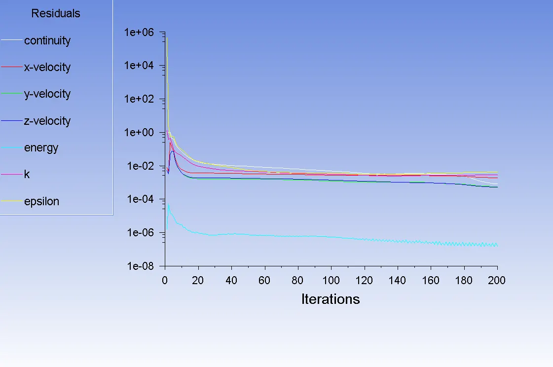
Fig4. Residual graph showing that energy residual curve is almost converged
 |
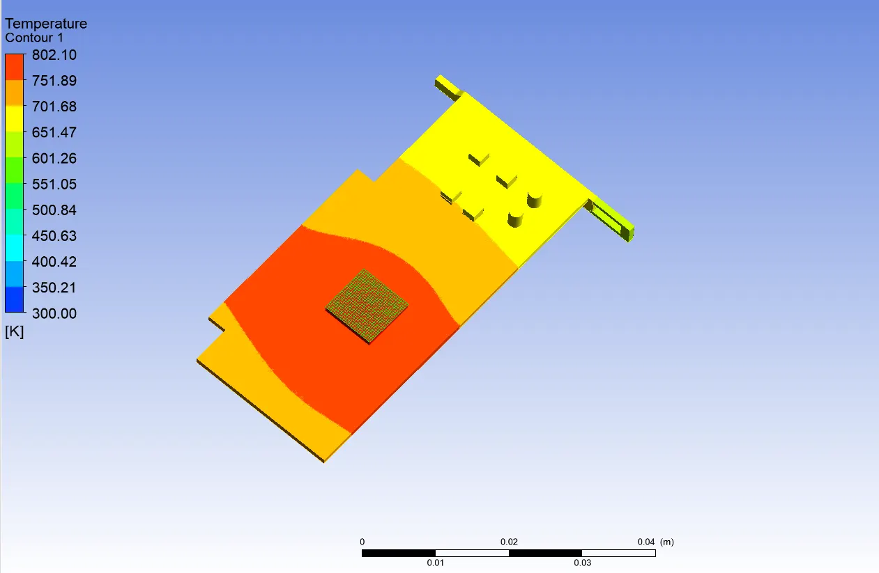 |
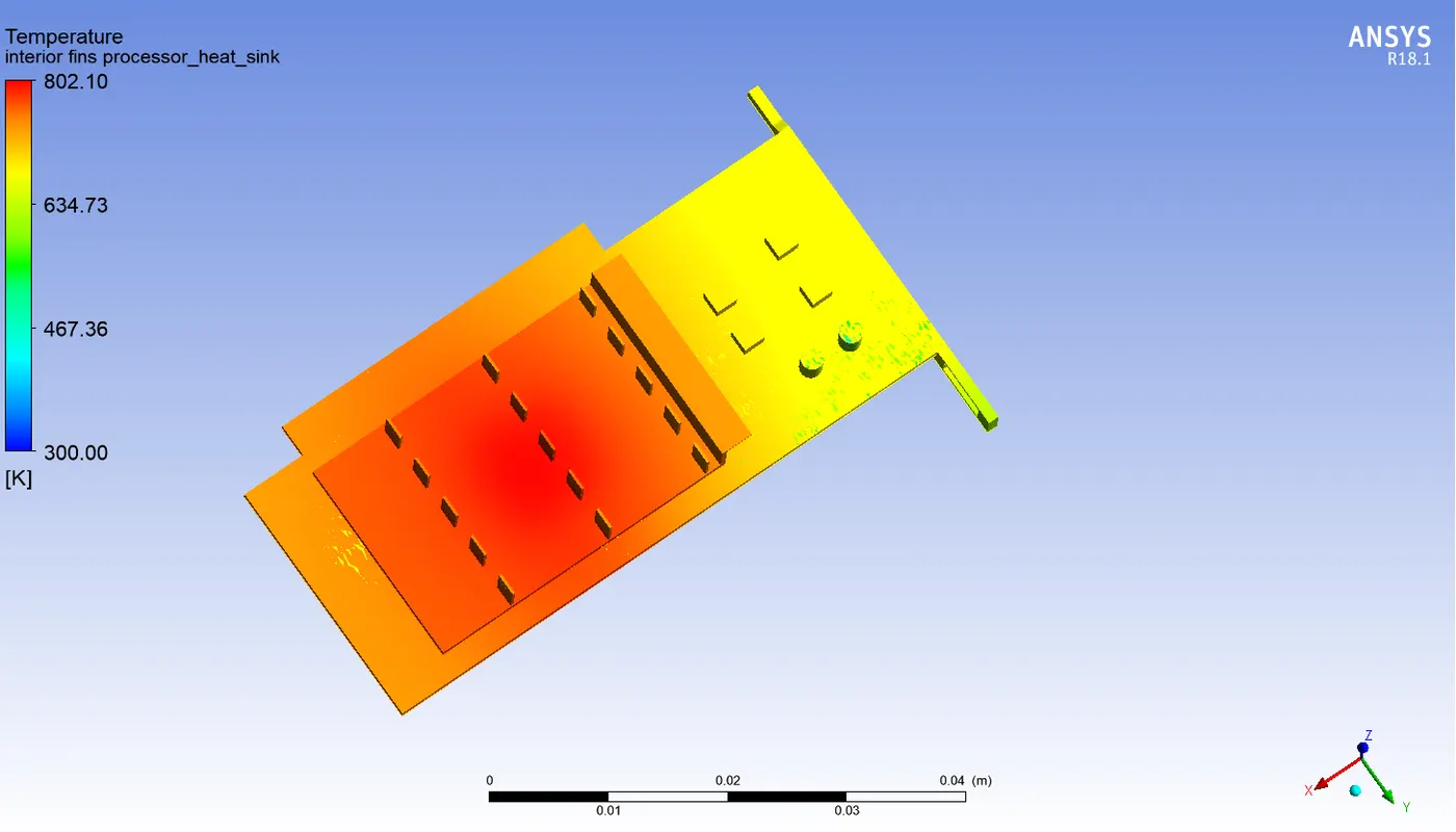
Fig5. Temperature contour on GPU showing max temperature of 802 k
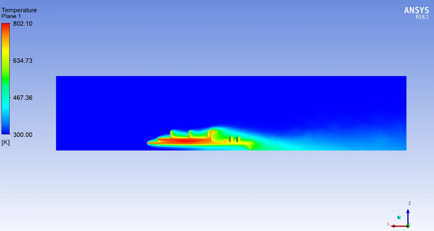
Fig6. Figure showing force convection via wind of velocity=1 m/s
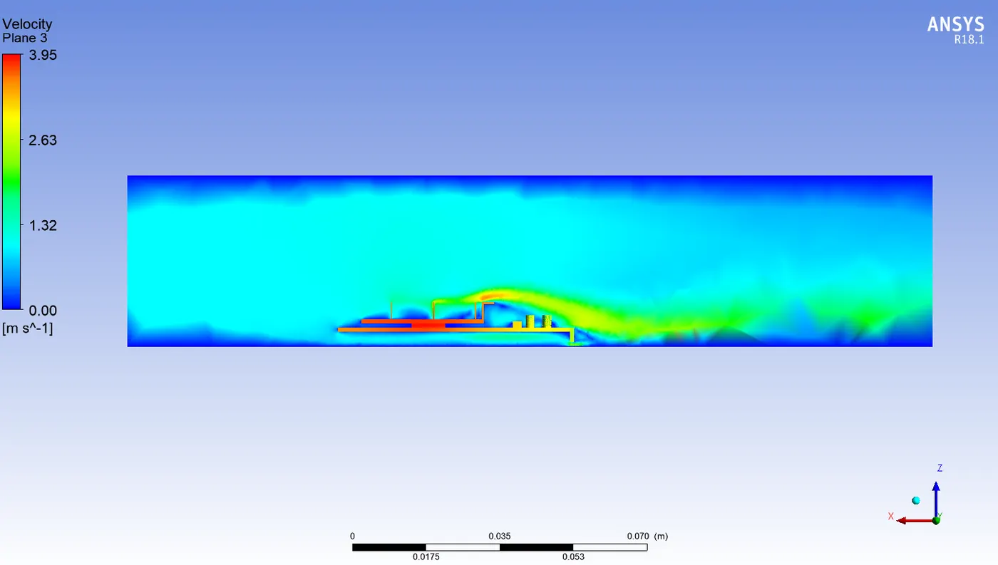
Fig7. Velocity contour of air flow over the GPU
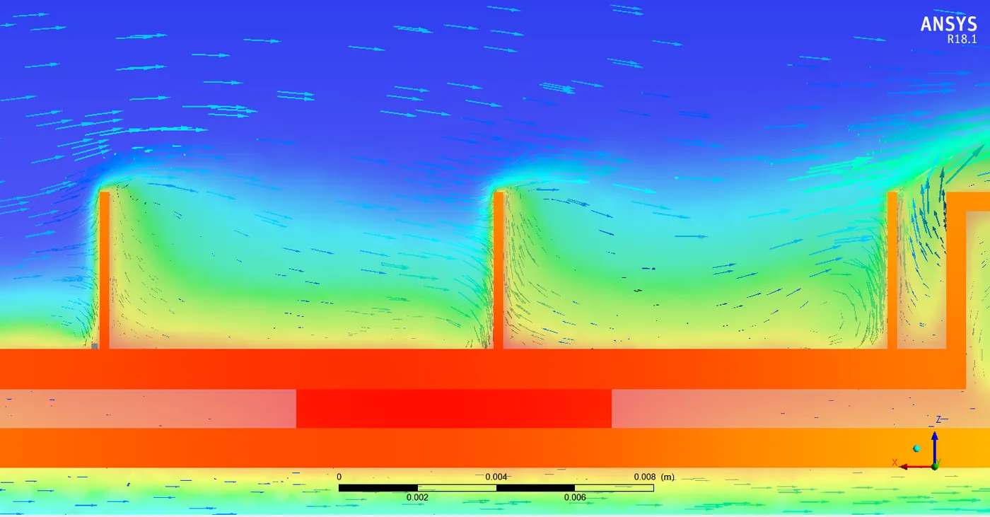
Fig8. Vector Representation of Velocity field

Fig9. maximum Wall Heat transfer coefficient
Maximum wall heat coefficient was found on the processor using virtual probe in Ansys post processing tool.
2. Velocity= 3 m/s
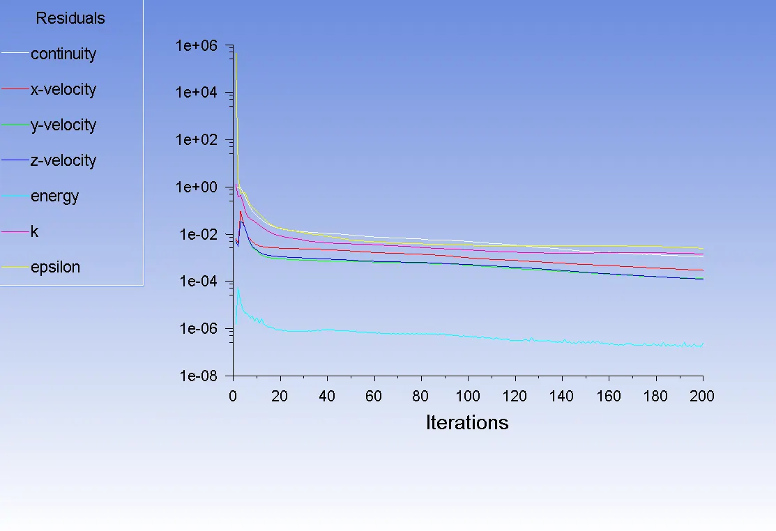
Fig10. Residual plot
 |
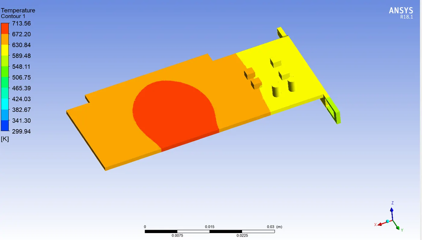 |
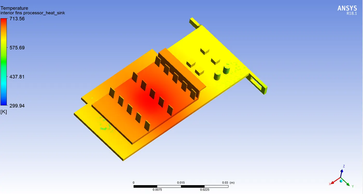
Fig11. Temperature contour of GPU component
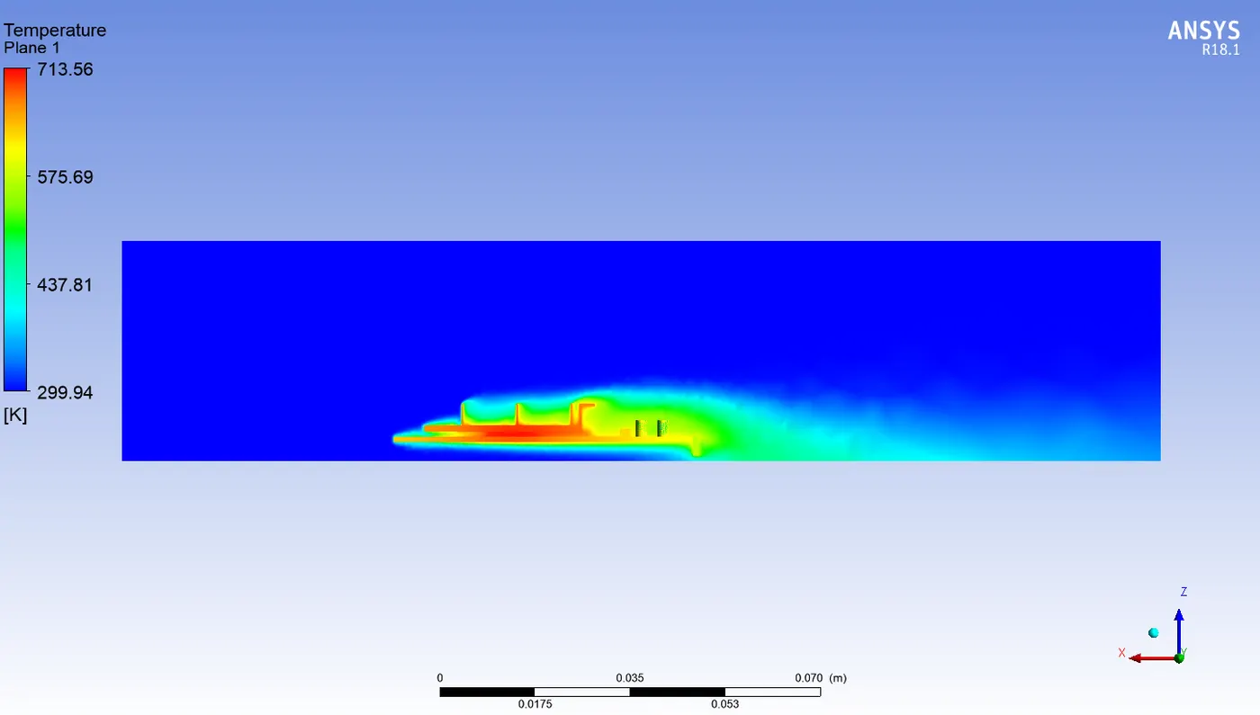
Fig12. Temperature contour on Monitor plane showing the effect of convection
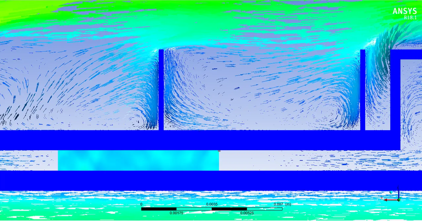
Fig13. Vector representation for more clarity of covection process
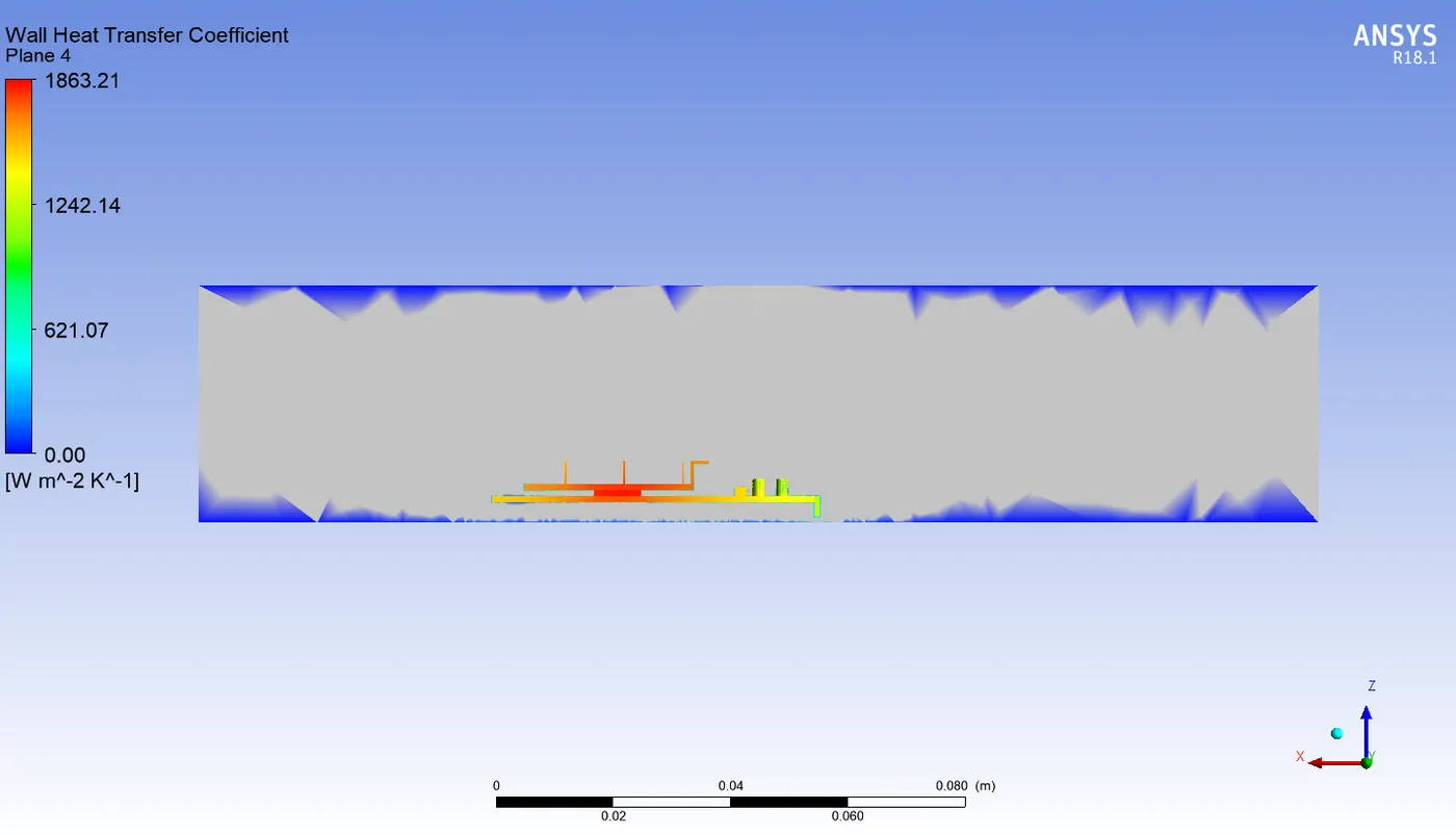
Fig14. Wall heat transfer coefficient
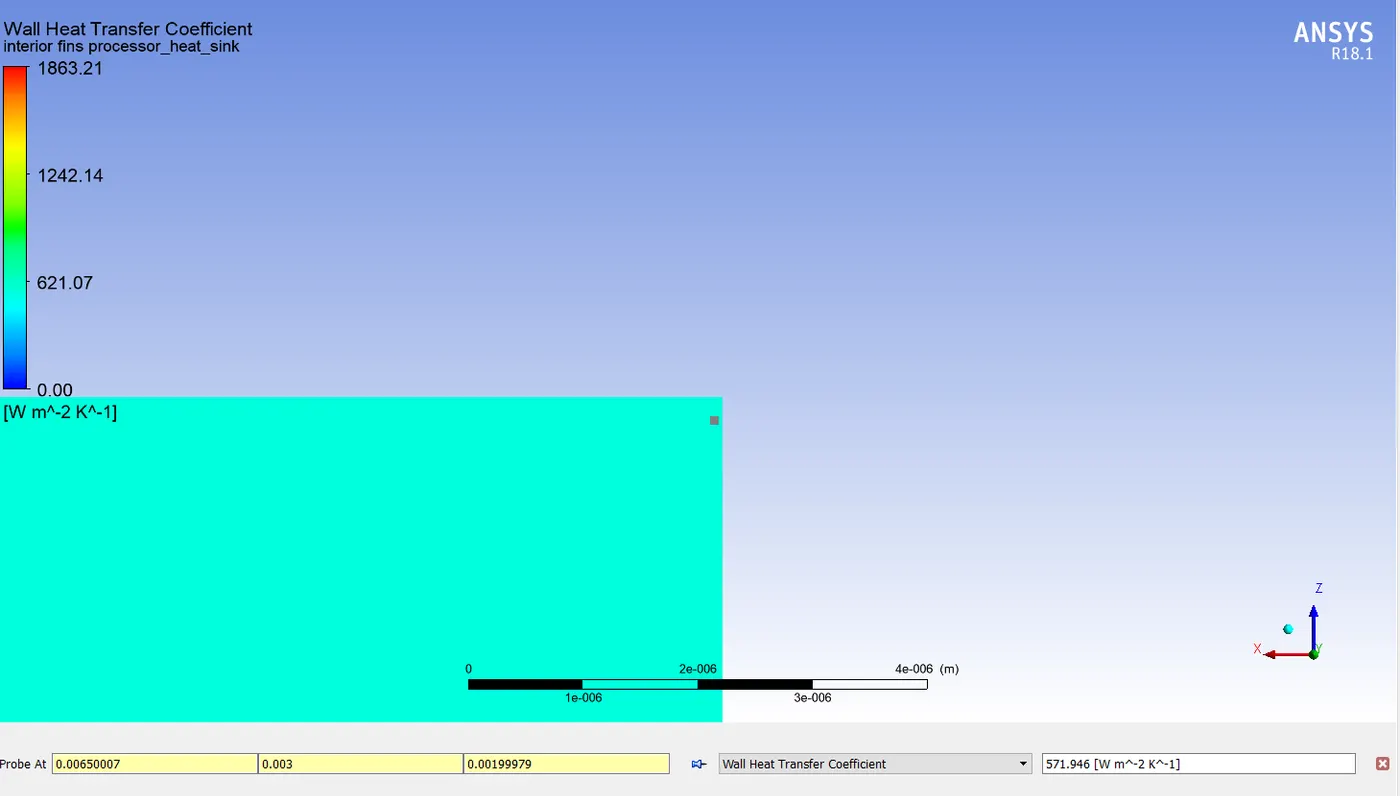
Fig15. Maximum wall heat transfer coefficient location using Probe
3. Velocity= 5 m/s
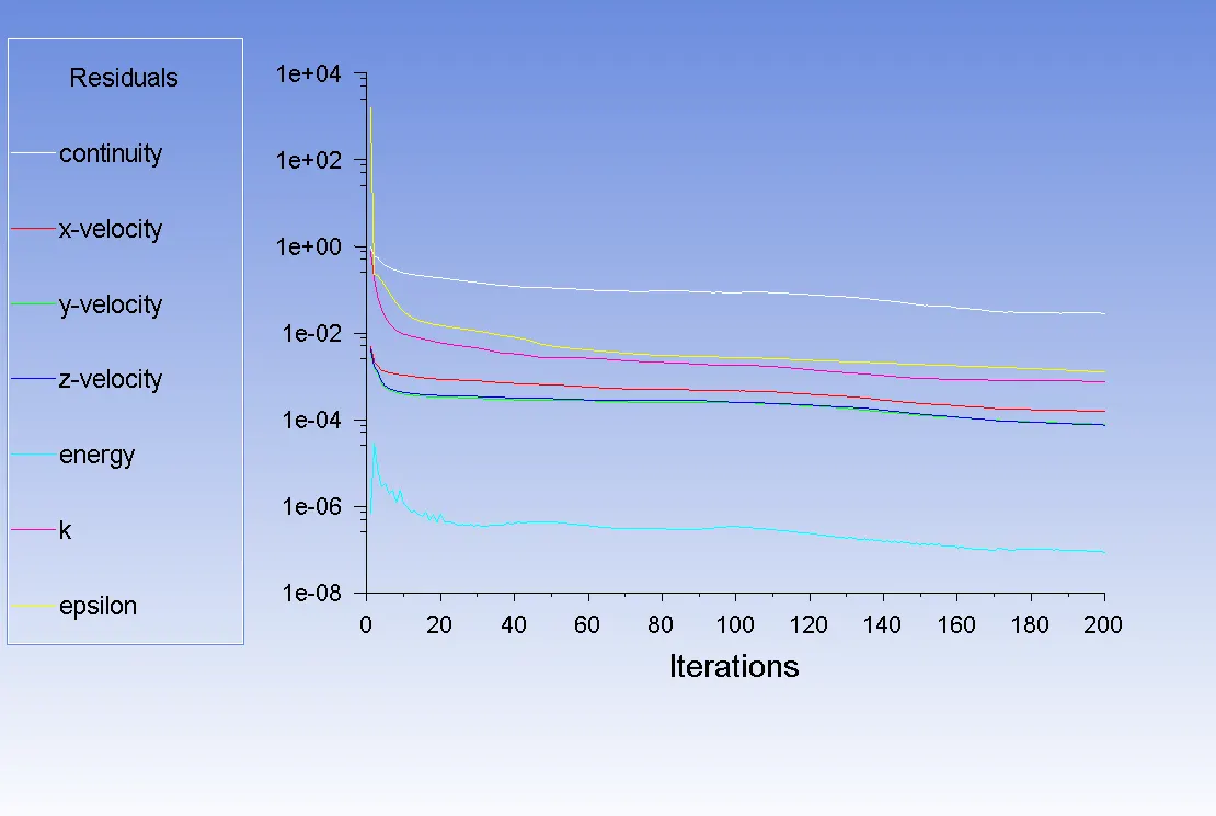
Fig16. Residual plot showing almost converged solution
convergence can be said if plot become flat with respect to x-axis that means it's not changing any more.
 |
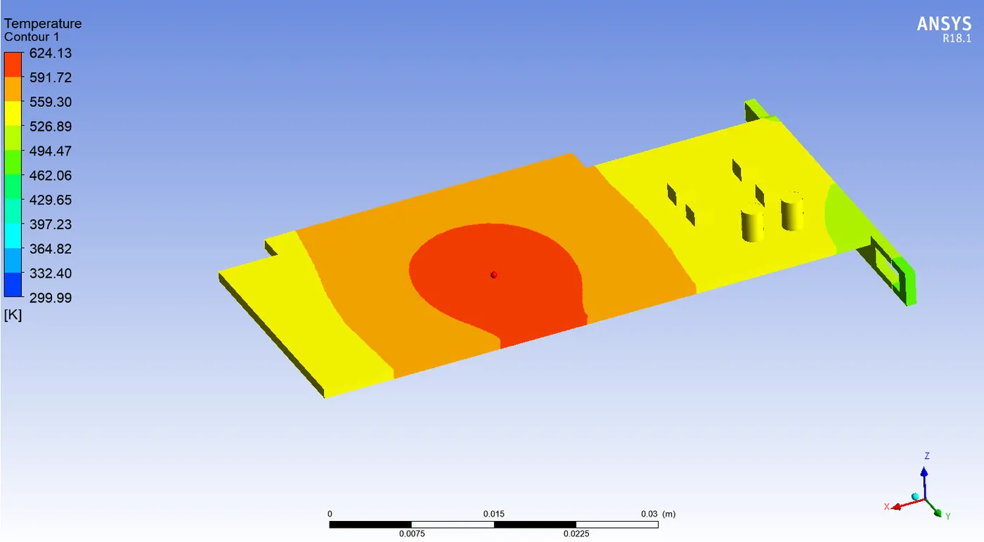 |
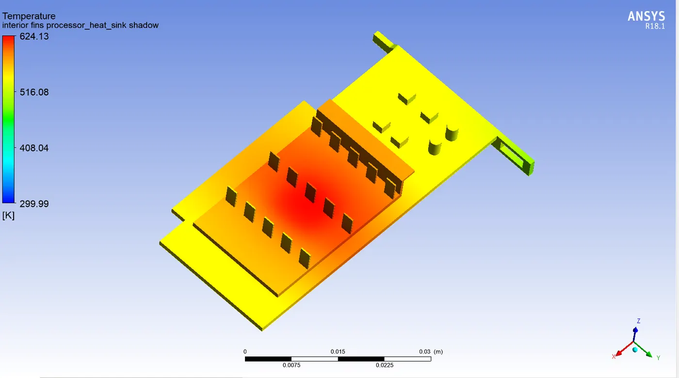
Fig17. Temperature contour
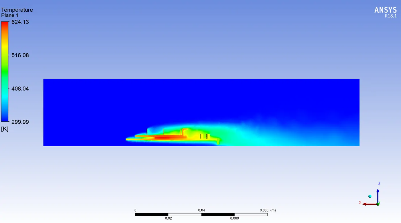
Fig18. Contour of temperature on plane showing convection effect
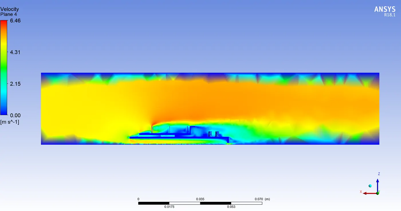
Fig19. Velocity contour
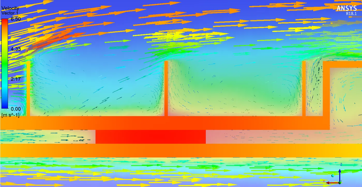
Fig20. Velocity vector over GPU
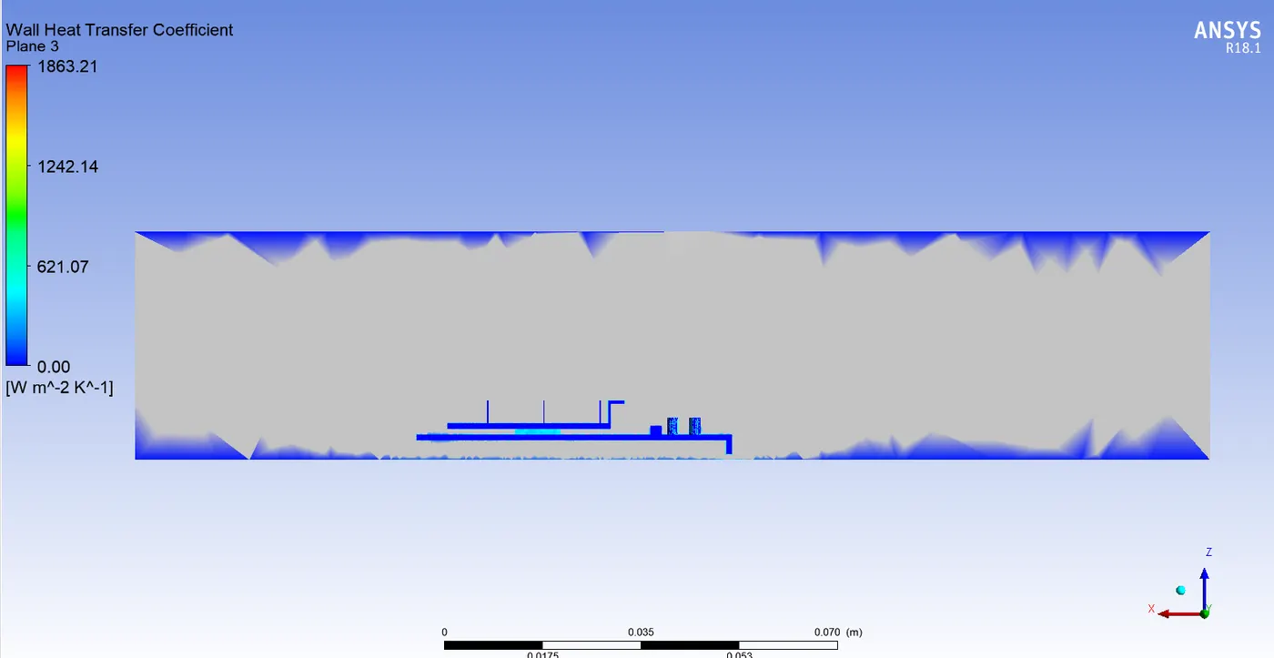
Fig21. Wall heat transfer coefficient contour
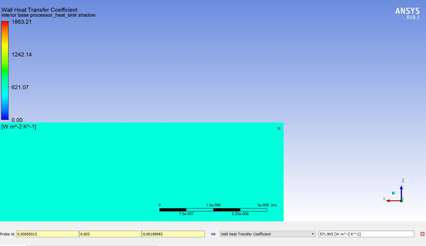
Fig22. Location of Max Wall heat transfer coefficient contour
Mesh Refinement
Fig22. Residual plot showing convergence
 |
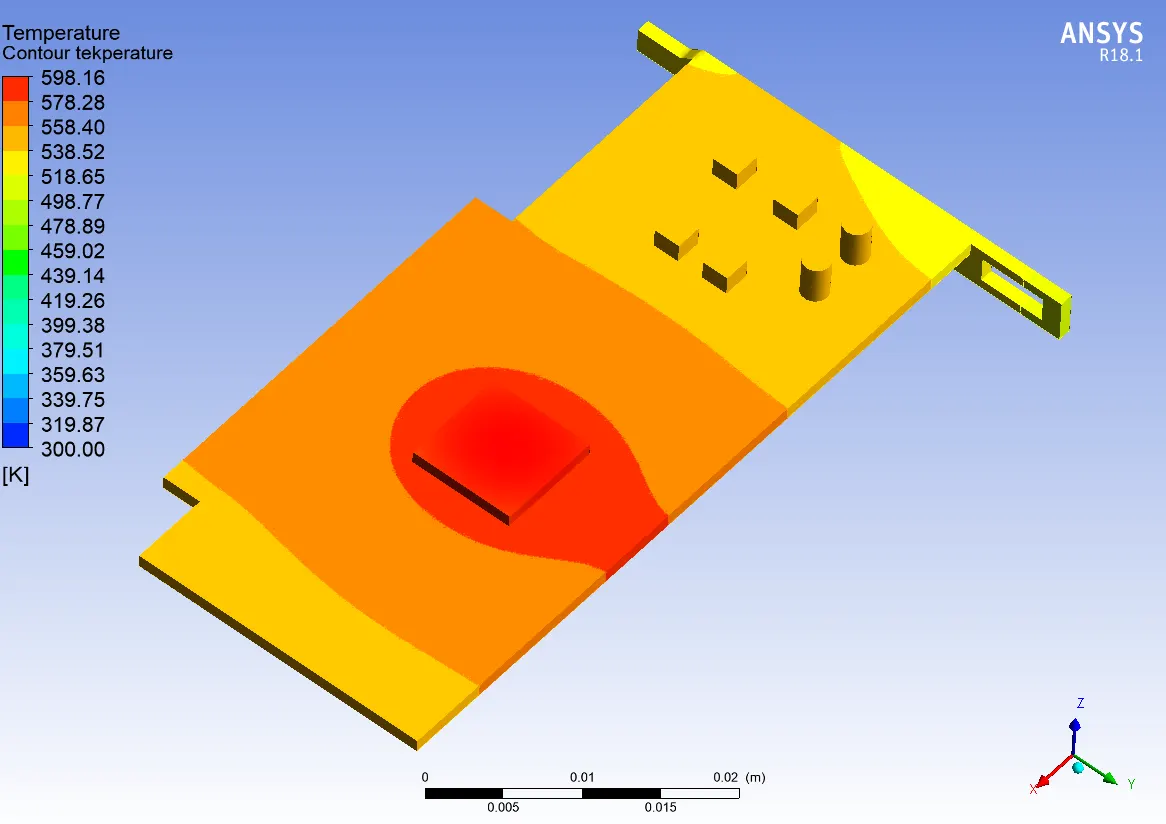 |
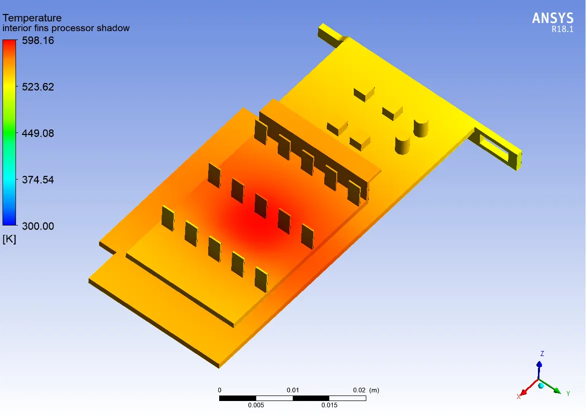
Fig23. Temperature contour on GPU
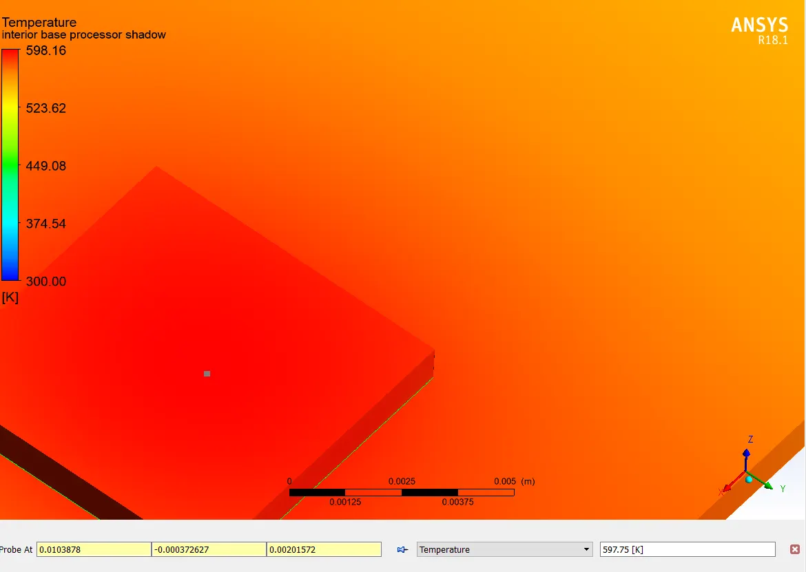
Fig24. Location of max temperature
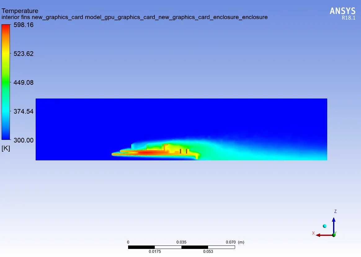
Fig25. Temperature contour on Plane showing Convection
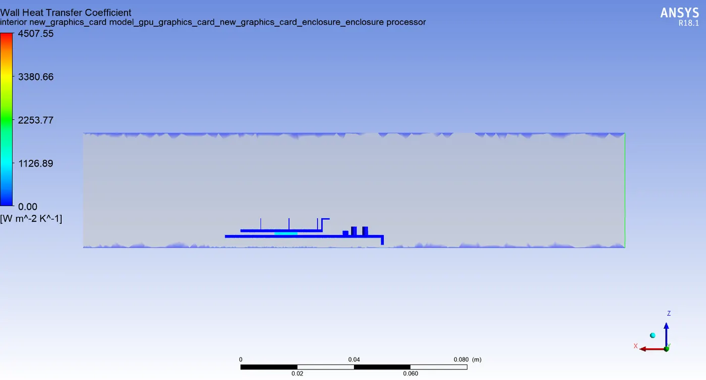
Fig26. Wall heat transfer coefficient contour
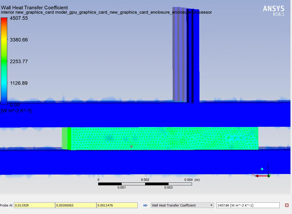
Fig27. Max wall heat transfer coefficient location
Observation and Analysis
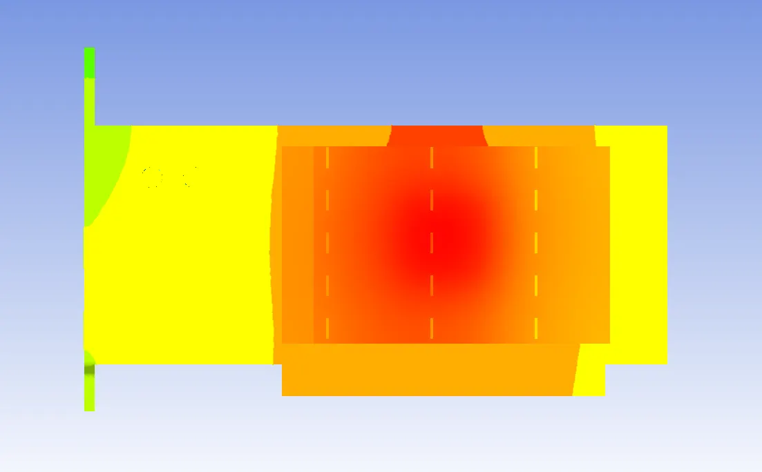
1. Temperature comparison between cases-
 |
 |
 |
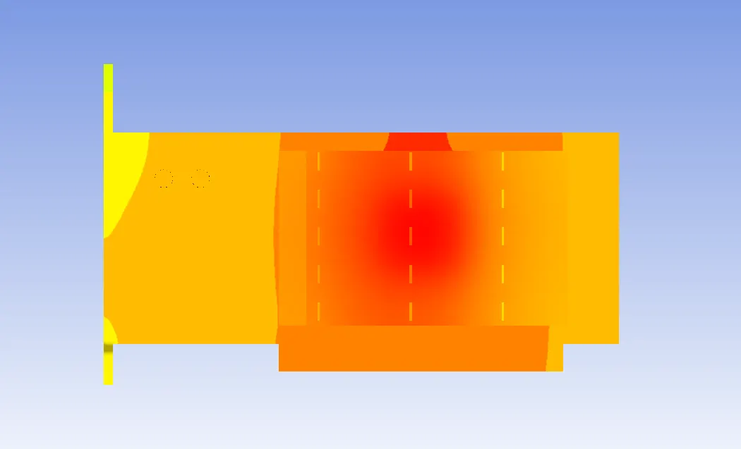 |
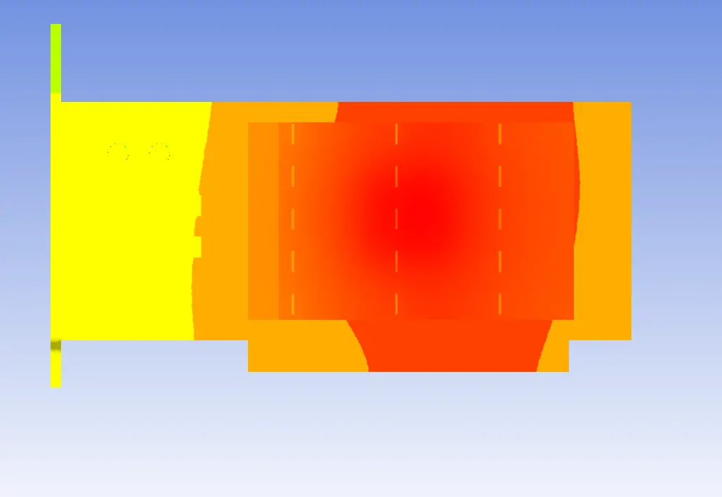
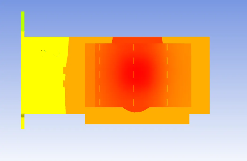
These are the contour of temperature of v=1, v=3, v=5 and mesh2 with v=5 respectively from left upper corner to right corner down.
| Cases | Max temperature |
| V=1 m/s | 802 k |
| V=3 m/s | 713.56 k |
| V=5 m/s | 624.13 k |
|
mesh2 V=5m/s |
598.16 k |
- These maximum temperature occur on the processor and this is very obvious as it acts as a heat source.
- The reson behind the decreased Temperature by increasing velocity is that which it make forced convection more efficiently.
2. Wall heat transfer Coefficient
Heat transfer Coefficient in Thermodynamics is the proporstionality constant between the heat flux and the thermodynamic driving force for the flow of heat (i.e., the temperature difference, ΔT).
| Cases | Max Value (W-m^2-K^-1) |
| V= 1m/s | 571.857 |
| V= 3m/s | 571.9446 |
| V= 5m/s | 597.75 |
|
Mesh2 V= 5m/s |
1407.86 |
- All these max value was occuring on the processor .
so we have seened that with a perticular GPU design we cooling effect can be enhanced by increasing fan speed.
References
[2]. https://en.wikipedia.org/wiki/Heat_transfer_coefficient
[3]. Fluid dynamics by Cengel cimbala