Conjugate Heat Transfer Analysis on a graphics card.

Aim:Perform a steady-state conjugate heat transfer analysis on a model of a graphics card.

Your Objectives:

1. Run the simulation by varying the velocity from 1m/sec to 5m/sec for at least 3 velocities and discuss the results.
2. Find out the maximum temperature and heat transfer coefficient attained by the processor.
3. Prove that the simulation has achieved convergence with appropriate images and plots.
4. Identify potential hotspots on the model.

Conjugate heat transfer is defined as the heat transfer between two domains by exchange of thermal energy. For a system the thermal energy available is defined by its temperature and the movement of thermal energy is defined by its heat flux through the outer walls. Heat transfer in solids happens through conduction and through the walls by convection and in liquid phase through convection.

CHT provides the temperature prediction and the hotspots regions at the solid liquidinterface and we can also predict the heat transfer accurately for example conduction through solids, convection through fluid and thermal radiation. It also provides the velocity and pressure distribution of the fluids moving inside in the solid. We can also use CHT in design optimisation for improvement for heat transfer and cooliing capacity.

Examples of Conjugate Heat transfer analysis:

HVAC, Heat Exchanger, Tank, Internal Combustion Engine, Heat Sink, Boiler, Reactor, Heat Pipe, Turbocharger.

Benefits:

Conjugate heat transfer analysis is beneficial in accurately predicting the surface temperatures and heat exchanging capabilities of the engineering devices. Through the analysis engineers can optimize the thermal characteristics for their chosen product design.

It can be used for following reasons.

1. Measurement of heat transfer through conduction in solid regions.
   
   
2. Identification of fluid flow parameters around the solid domain.
   
   
3. Measurement of convective heat transfer from solids to surrounding fluid environment.
4. Evaluation of heat transfer capabilities of the product.
   
   
5. Measurement of surface temperatures and hot spot regions.
6. Design optimization for improvement in heat transfer rate and cooling capacity.

Details of some applications.

Turbocharger:

The figure below depicts the various heat sources, sinks and paths in diesel enginer turbocharger.Turbocharger which comprises of turbine stage and compressor stage has various sources of heat generation and these requires cooling, which is carried away means of convective heat transfer where fluid such as oil, coolant or air is circulated. CHT analysis can be used to calculate compressor heat efficiency value and estimate the quantities of heat which enter and leave the respective stages both before and after compression. The image below show the CHT model of a Cummins non-water cooled HE200VG turbocharger, generated in order to investigate compressor stage performance at several running points when considering heat transfer across the housings and core components.

Shell and Tube type Heat exchanger:

Shell and Tube type heat exchangers are most commonly employed heat exchangers in industry where one fluid runs from the inside of the tubes and another fluid runs over the tube and heat transfer takes place.

CHT analysis of Heat exchangers allows along with CFD allows

1. Effective Prototyping during HeatExchanger design phase.
2. Visualization of flow patterns and alter the geometry of the HEx to suit the temperature requirements.
3. Enhance Baffle designs to reduce system pressuredrop, choosing an optimized shape and weight for the shell casing.
4. Simulation of complex processes such ascondensation and vapourisation inside the system.

CHT Analysis of Exhaust Manifold.

In the following project CHT analysis on exhaust manifold is carried out to find out velocity, temperature and heat transfer coefficient. Two simulations with baselinemesh and refined mesh are carried out and compared.

Case set-up:

Geometry:

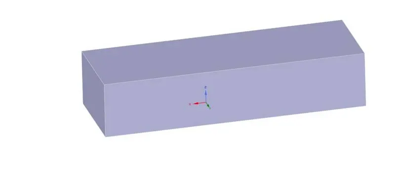
Enclosure:

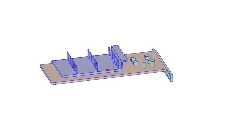
Fins,processor and baseline:

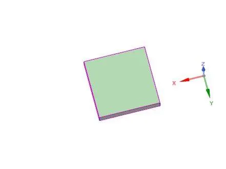
Processor:

Fins: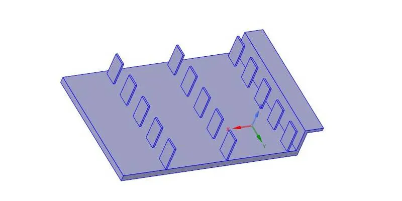

Meshing:

Coarse mesh:

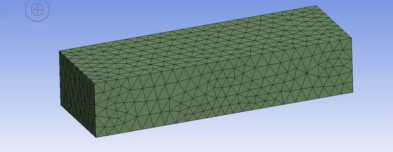
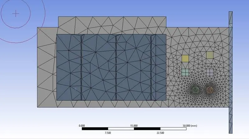
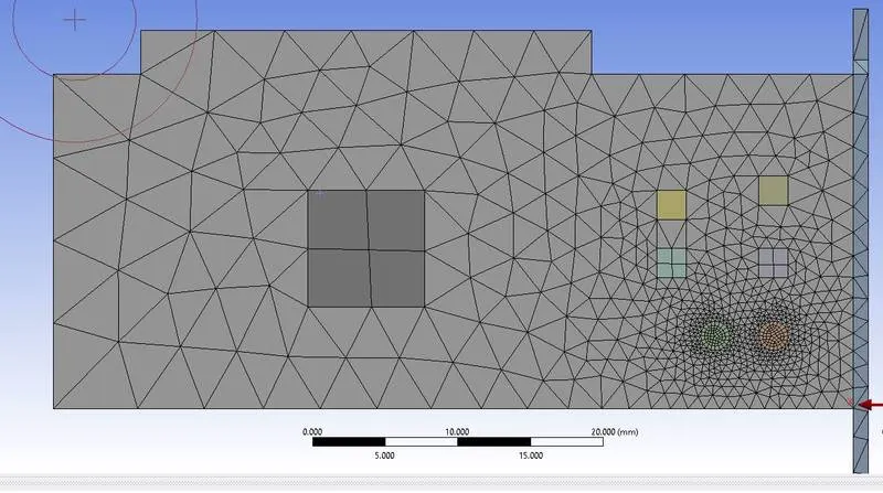
Element size=8.4521mm

Nodes=16265

Elements=86510.

Set-up:

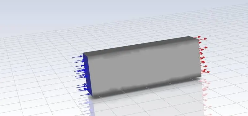
Setting up the physics :

Setting up the physics for CHT analysis on a graphics card in ANSYS fluent.

• For this case we are using pressure-based steady state solver
• Velocity formulation - Absolute

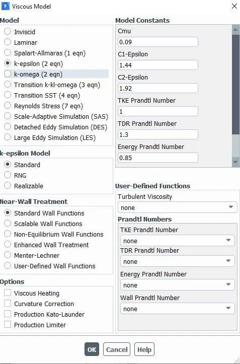
Models setup

• Energy
• Viscous - k-epsilon

Materials :

We are using different material for all the component

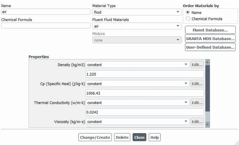
For fluid : Air (Flowing inside the domain)

• Density = 1.225 kg/m^3
• Viscosity = 1.7894e-05 kg/ms

For Fins : copper(Graphics card component)

• Density = 8978 kg/m^3
• Specific heat = 381 j/kg-k
• Thermal conductivity = 387.6 w/m-k

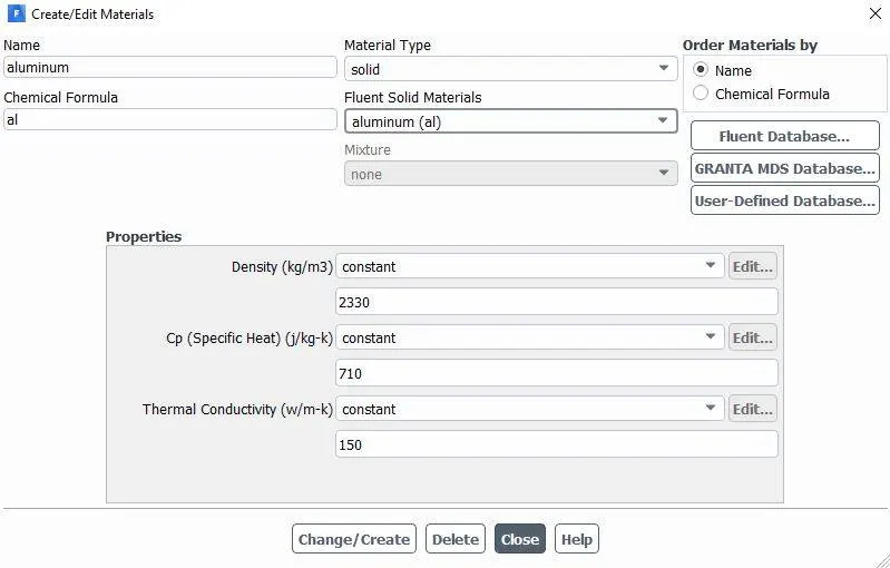
For Processor : aluminium(Graphics card component)

• Density = 2330 kg/m^3
• Specific heat = 710 j/kg-k
• Thermal conductivity = 150 w/m-k

For Base : steel (Graphics card component)

• Density = 8050 kg/m^3
• Specific heat = 502 j/kg-k
• Thermal conductivity = 16.27 w/m-k

Setting up the source terms :

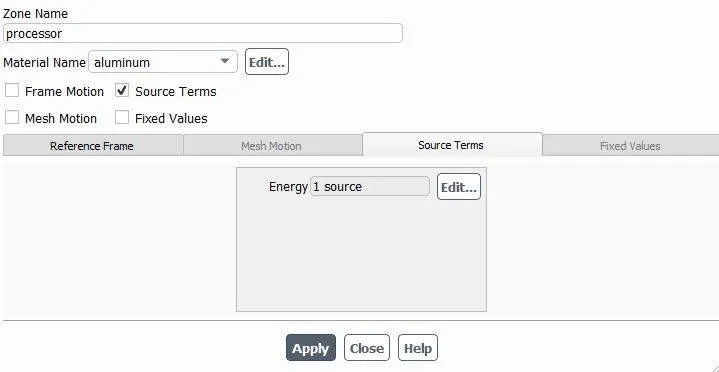
For this case we consider that, our processor is a source terms and it generating heat.

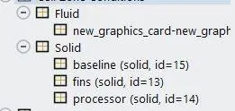
So, for setting up the source term go to Zones - Cell zones - and click on the processor for editing which is in the Solid.

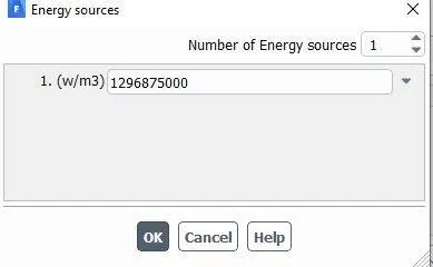
After that select the material to gold and click on the source terms to enabled it and set the energy source to 1.

Calculation for the Energy source

Let the processor consume 83 W of power to work.

Dimension of the processor = 8*8*1 mm^3

So, Energy produced by the processor is 1296875000 w/m^3.

Inlet

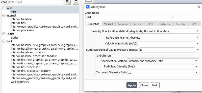
• Air is used as a fluid
• Velocity = 1 m/s
• Temperature = 300 K

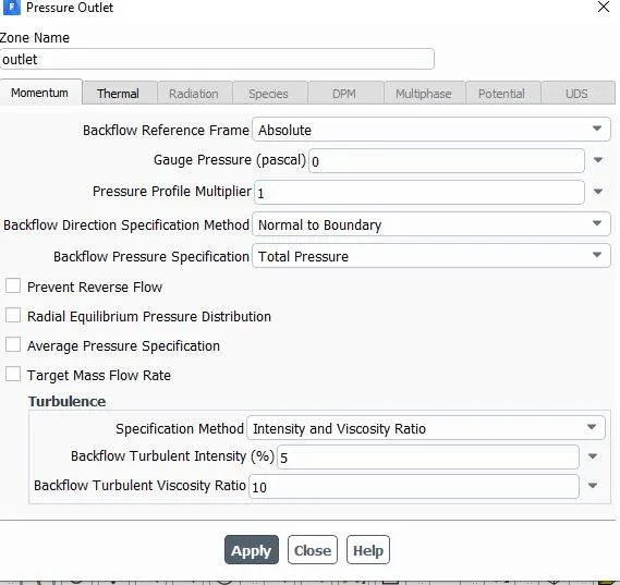
Outlet

• Pressure = Gauge pressure (0 pa)

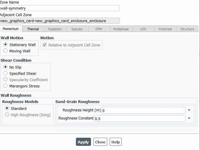
All the four side faces

• Follow the symmetry B/C

Graphics card

• Follow the No slip Wall B/C

Results:

Residuals:

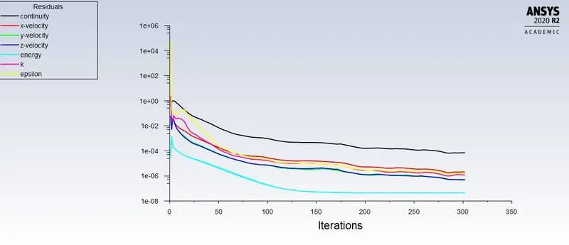
Here convergence is taking place after 220 iterations.

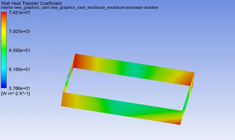
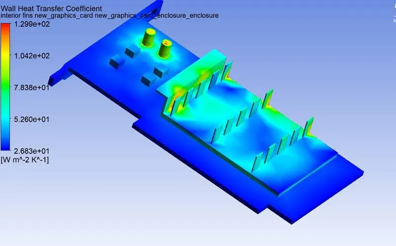
Heat transfer co-efficient attained by processor:

Maximum temperature attained by the processor:

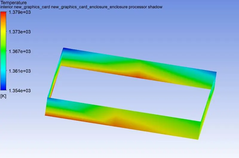
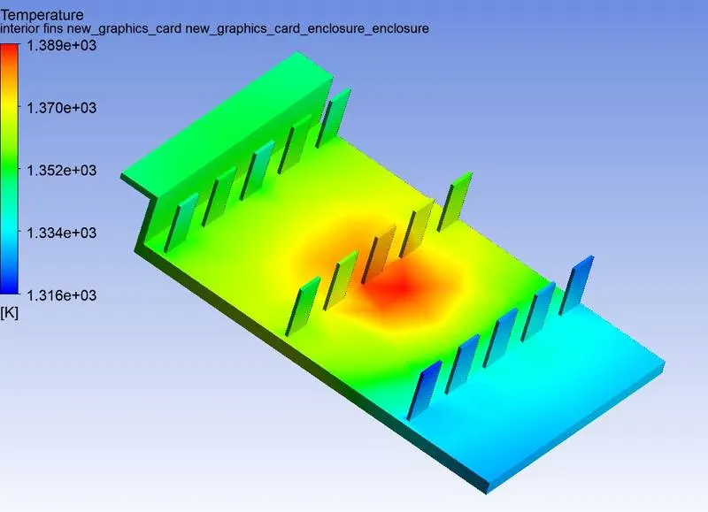
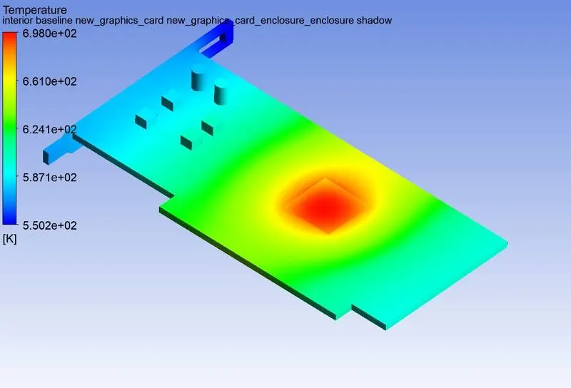
Potential hotspot on the fin:

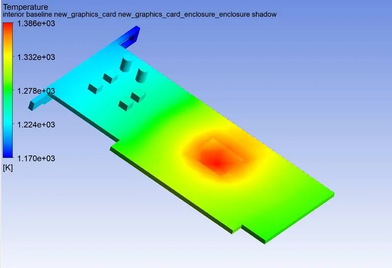
Potential hotspot on the baseline:

Refined mesh:

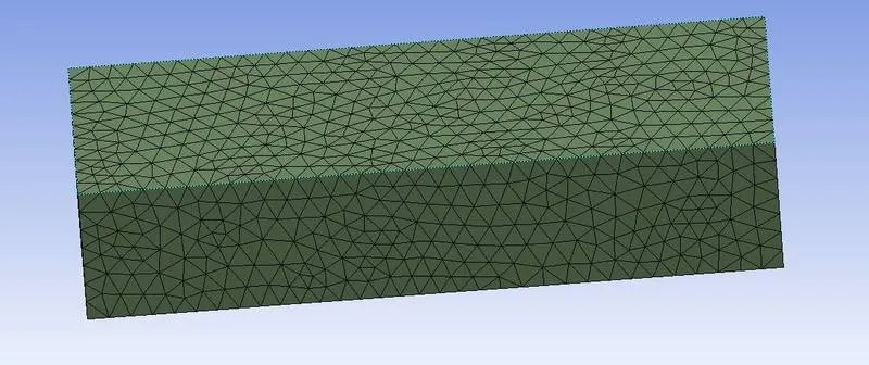
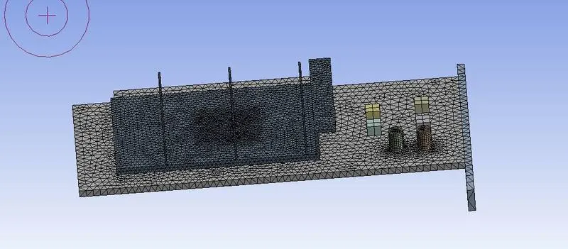
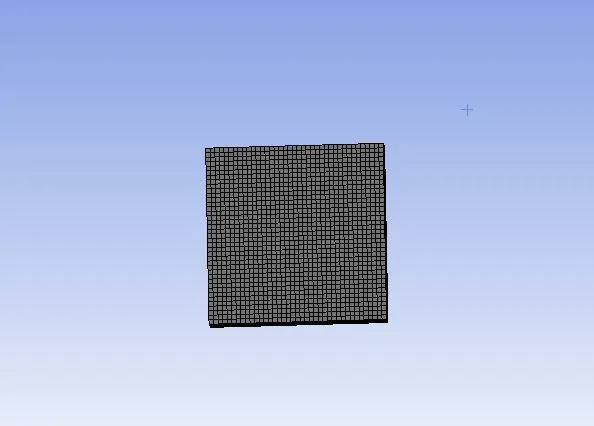
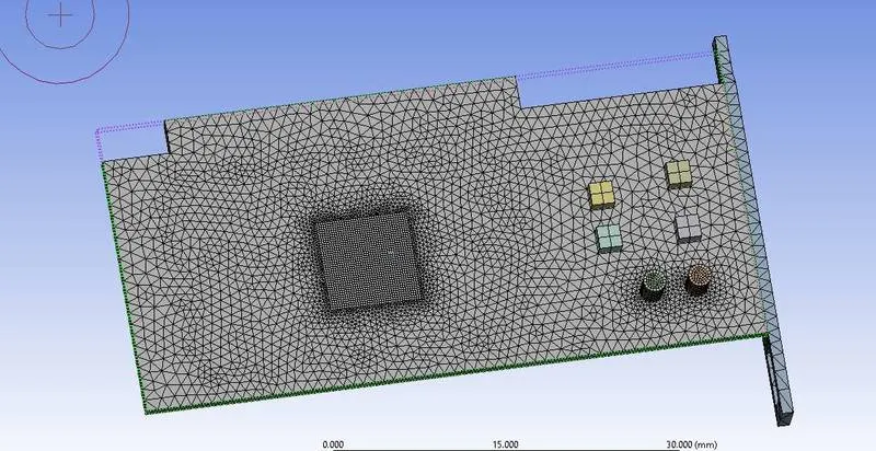
Element size for enclousre=6 mm

Element size for fins=0.6 mm

Elemtent size for processor=0.2 mm

Element size for baseline=1 mm

Nodes=85780

Elements=455430.

CASE 1: for velocity 1 m/s .

Residuals:

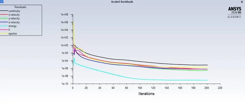
Here convergence is taking place after 150 iterations.

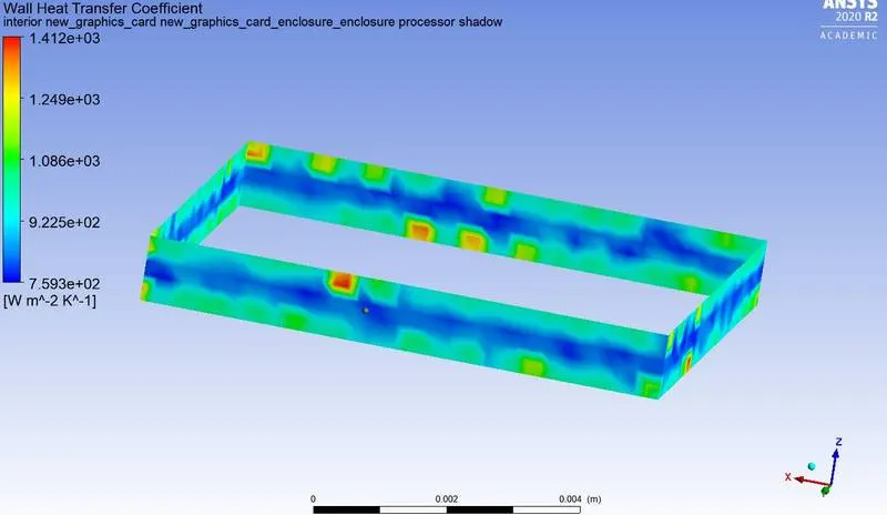
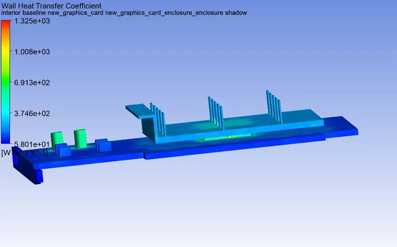
Heat transfer co-efficient attained by processor:

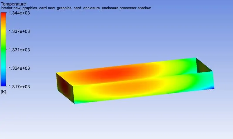
Maximum temperature attained by the processor:

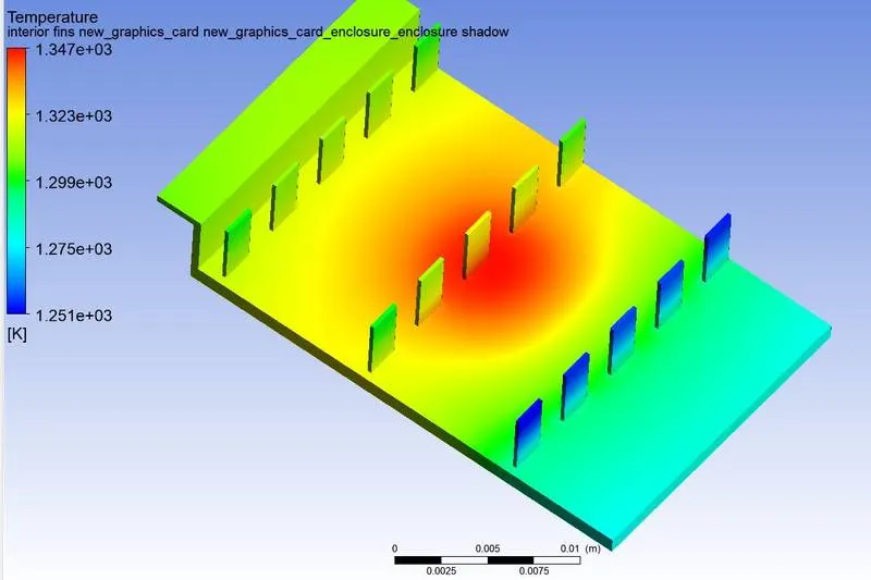
Potential hotspot on the fin:

Potential hotspot on the baseline:

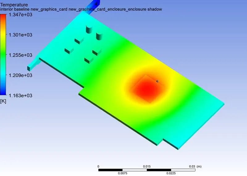
CASE 2 :for velocity 3 m/s.

Residuals:

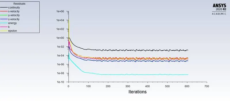
Here convergence is taking place after 250 iterations.

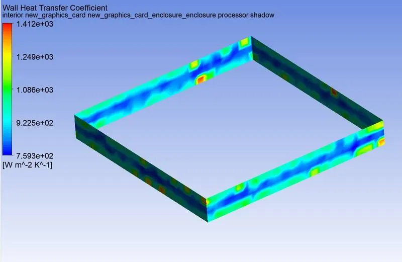
Heat transfer co-efficient attained by processor:

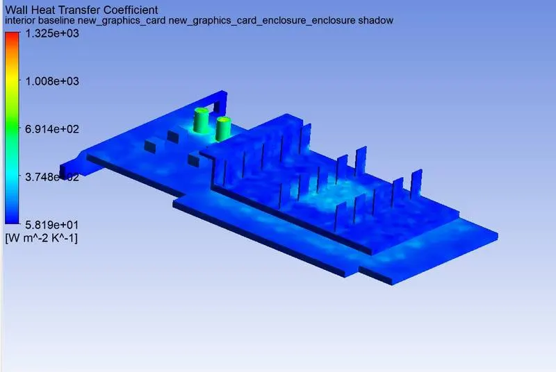
Maximum temperature attained by the processor:

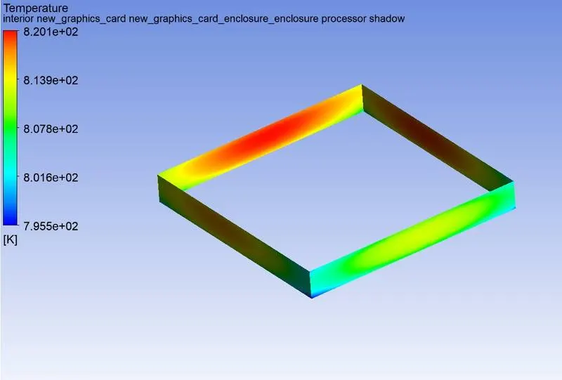
Potential hotspot on the fin:

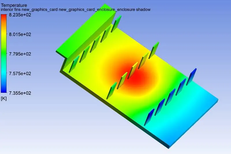
Potential hotspot on the baseline:

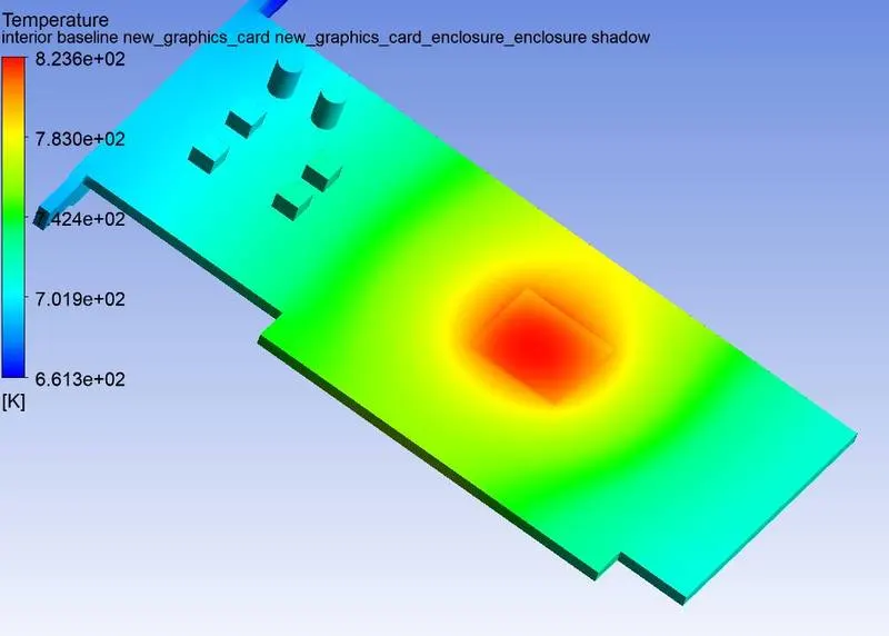
CASE 3 :for velocity 5 m/s.

Residuals:

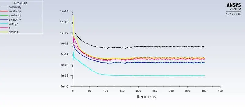
Here convergence is taking place after 200 iterations.

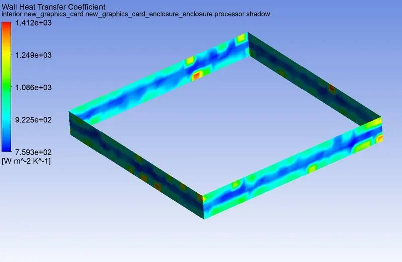
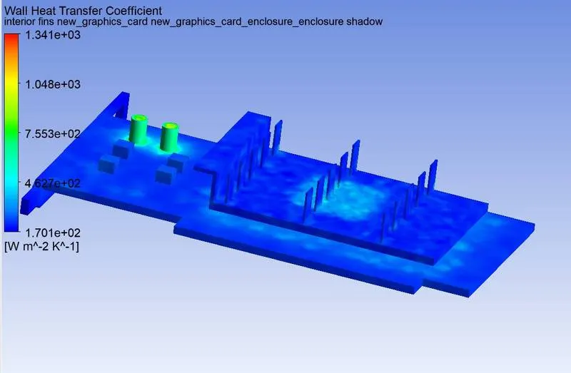
Heat transfer co-efficient attained by processor:

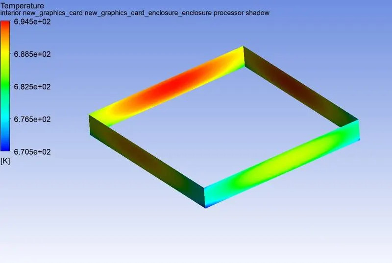
Maximum temperature attained by the processor:

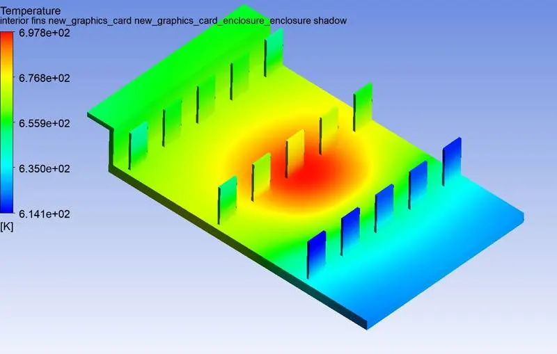
Potential hotspot on the fin:

Potential hotspot on the baseline:

Results:

Type of mesh used	Fluid flow velocity(m/s)	Maximum temperature(K)	Maximum wall heat transfer coefficient(W/m^2 K)
Coarse	1	1379	74.20
Refined	1	1343	1412
Refined	3	820	1412
Refined	5	694	1412

From the above table, we can say that the refined mesh gives more accurate results compared to the coarse mesh. The maximum temperature of the graphic card assembly reduces with the increase in the flow velocity. This is because as the velocity of flow is increased, more amount of heat is carried away by air. The heat transfer coefficient is the highest in the regions which are in contact with the processor. This region is not affected by the change in flow velocity since there is no airflow present, hence, the maximum heat transfer coefficient remains the same for all the flow velocities. But this does not mean that the maximum wall heat transfer coefficient remains the same in the regions exposed to the fluid flow. In the regions which are exposed to the fluid flow, the wall heat transfer coefficient increases with the increase in fluid flow velocity.

Conclusions:

1. The refined mesh provides more accurate results compared to the coarse mesh. This accuracy can be increased by increasing the number of mesh elements.
2. The temperature of the graphic card assembly decreases with the increase in fluid flow velocity because as the velocity of flow increases, more heat is carried away by it, hence cooling the graphic card.
3. The highest wall heat transfer coefficient was obtained near the processor walls, which is 1412 W/m^2K. This region is not affected by the fluid flow, since these walls are in contact with each other and there is no space for air to flow in between them. In the regions which experience fluid flow, the wall heat transfer coefficient increases with the increase in fluid flow velocity.
4. The processor is the potential hotspot of the graphic card assembly since it is the only heat generating part of the entire assembly. The temperature and wall heat transfer coefficients of the processor and other parts are influenced by the heat generated by the processor. Also, the heat generated by the processor depends on its workload. Higher the workload, the higher the heat generated by the processor.