Challenge on Combustion

INTRODUCTION

The most important and common way in which energy is released is by combustion. Combustion is a process in which a fuel combines with an oxidizer to release energy and produces some products of combustion known as the exhaust. If a hydrocarbon-based fuel is burned in oxygen alone the products of combustion will be carbon dioxide and water. If the same fuel is burned in the air which contains oxygen and nitrogen there will be oxides of nitrogen also in the product of combustion. Since the temperature of the exhaust is high the exhaust products will be in gaseous state but there can be liquid or solid exhaust products as well. Soot is a solid exhaust product found in some combustion process. The exhaust produced in a combustion process is harmful to health and the environment. Therefore it is important to predict the concentration of the exhaust products developed using computer simulations.

The production of soot can be attributed to fuel-rich condition, high temperature etc. which will have an adverse effect on the combustion device and also contribute to the reduction in its efficiency. The stringent government policies on emission standards also make it very important that we create a detailed understanding of the exhaust products. However, the uncertainty increases significantly while modelling the soot formation. The mechanisms involved in soot formation process are strongly coupled with mixing and radiative heat transfer and depend on soot volume fraction itself, make the prediction of soot emissions a challenging task, leading to large errors in exhaust concentration even with small mispredictions in the formation rates. In methane-air flames, the soot-production takes place from small species like acetylene that grow to form polyaromatic hydrocarbons (PAH) and eventually soot. However, practical fuels such as kerosene contain aromatics, which significantly accelerate the soot formation process. The models developed for methane-air mixture cannot be used for practical fuels like gasoline or diesel for modelling the soot formation.

In this study, we have used FLUENT module in the ANSYS 2020 R1 software to model the emissions from a combustor which uses a methane-air mixture. The `NO_x` emissions from the combustor is a pollutant and a greenhouse gas. A model is tested where water is added to the fuel from 5% to 30% of the mole fraction and the effect on the formation of `NO_x`. In practice the `NO_x` formed when the hydrocarbon fuel is burned are `NO`and `N_2O` where 90% is attributed to `NO`. So while modelling the emissions the only oxides of nitrogen that needs to be modelled are the `NO` and `N_2O`. Nitrogen is a reasonably stable element which reacts only at very high temperature. A very high temperature can be achieved when the fuel is in the stoichiometric composition. The fuel is made lean by adding water, and it also helps in reducing the temperature, thereby reducing the emission of `NO_x`.

AIM

Perform a combustion simulation on the combustor model and plot the variation of the mass fraction of the different species in the simulation using line probes at different locations of the combustor. The plots for emissions of `CO_2`, `H_2O`, `CH_4`,`N_2`, `O_2`,`NO_x`& Soot formation needs to be made at different locations.

The water content in the fuel from 5% to 30% by mole and observe the effect of it on the results. It is necessary to provide line plots and contours to prove that as the wat`S_\phi = 0`er content is increased the soot and `NO_x` formation is reduced.

THEORY AND THE MATHEMATICAL MODEL

The governing equations that need to be solved are the transport equation and the model equation which are used to predict turbulence. A general form of the equation which needs to be solved is given below for a general dependent variable `\phi`:

\begin{equation}
\frac{\partial(\rho \phi)}{\partial t}+\frac{\partial\left(\rho u_{z} \phi\right)}{\partial z}+\frac{1}{r} \frac{\partial\left(r \rho u_{r} \phi\right)}{\partial r}=\frac{\partial}{\partial z}\left(\Gamma \frac{\partial \phi}{\partial z}\right)+\frac{1}{r} \frac{\partial}{\partial r}\left(r \Gamma \frac{\partial \phi}{\partial r}\right)+S_{\phi}
\end{equation}

Where `\Gamma` is the diffusion coefficient for variable `\phi` and`S_{phi}` is the source term for variable `\phi`.

For the continuity equation `\phi =1`, `\Gamma = 0` and `S_{phi}=0`.

For r momentum equation `\phi =u_r`, `\Gamma = \mu_{eff}` and `S_{phi}=
-\frac{\partial p}{\partial r}-\mu_{e f f} \frac{u_{r}}{r^{2}}+S_{t}^{r}`.

For z momentum equation `\phi =u_z`, `\Gamma = \mu_{eff}` and `S_{phi}=
-\frac{\partial p}{\partial z}+S_{t}^{z}
`.

Where `S_{t}^{r}` and `S_{t}^{z}` are the turbulent source terms which can be defined as

\begin{equation}
S_{t}^{r}=\left(\begin{array}{l}
\frac{\partial}{\partial z}\left(\mu_{e f f} \frac{\partial u_{z}}{\partial r}\right)+\frac{1}{r} \frac{\partial}{\partial r}\left(r \mu_{e f f} \frac{\partial u_{r}}{\partial r}\right)-\mu_{e f f} \frac{u_{r}}{r^{2}}
-\frac{2}{3} \frac{\partial}{\partial r}\left(\mu_{e f f} \nabla \cdot \mathbf{V}+\rho k\right)
\end{array}\right)
\end{equation}

and

\begin{equation}
S_{t}^{z}=\left(\begin{array}{l}
\frac{\partial}{\partial z}\left(\mu_{e f f} \frac{\partial u_{z}}{\partial z}\right)+\frac{1}{r} \frac{\partial}{\partial r}\left(r \mu_{e f f} \frac{\partial u_{r}}{\partial z}\right)
-\frac{2}{3} \frac{\partial}{\partial z}\left(\mu_{e f f} \nabla \cdot \mathbf{V}+\rho k\right)
\end{array}\right)
\end{equation}

The turbulence model employed in this simulation is the `k-epsilon` model where k represents the turbulent kinetic energy and `\epsilon` represents the turbulent dissipation rate.

For modelling the turbulent kinetic energy equation, `\phi =k`, `\Gamma = \frac{\mu_{eff}}{\sigma_{k}}` and `S_{phi}=G-\frac{2}{3}(\mu_{e f f} \nabla \cdot \mathbf{V}+\rho k) \nabla \cdot \mathbf{V}-\rho \varepsilon`.

For modelling the turbulent dissipation equation, `\phi =\epsilon`, `\Gamma = \frac{\mu_{eff}}{\sigma_{\epsilon}}` and `S_{phi}=\frac{\varepsilon}{k}(C_{1} G-C_{2} \rho \varepsilon)`.

Where G is the turbulent kinetic energy production which can be modelled as:

\begin{equation}
G=\mu_{t}\left(\frac{\partial u_{z}}{\partial r}+\frac{\partial u_{r}}{\partial z}\right)^{2}+2 \mu_{t}\left(\left(\frac{\partial u_{z}}{\partial z}\right)^{2}+\left(\frac{\partial u_{r}}{\partial r}\right)^{2}+\left(\frac{u_{r}}{r}\right)^{2}\right).
\end{equation}

Since the above equation deals with combustion it is important to solve the energy equation. For the energy equation `\phi =h`, `\Gamma = \frac{\mu_{eff}}{\sigma_{n,t}}` and `S_{phi}=\frac{\partial p}{\partial t}`

For the chemical reaction `\phi =m_f`, `\Gamma = \frac{\mu_{t}}{\sigma_{n,t}}` and `S_{phi}=-R_f`

The total enthalpy can be defined as \begin{equation}
h=C_{p} T+\frac{1}{2}\left(u_{r}^{2}+u_{z}^{2}\right)+k+\sum m_{j} h_{j}
\end{equation}

where `\sum_{\text {all } j} m_{j}=1`. The effective viscosity can be drfined as `\mu_{eff}=\mu_{t}+ \mu`, and the turbulent viscosity `\mu_t = \frac{C_{\mu}\rho k^2}{\epsilon}`.

`\nabla \cdot \mathbf{V}=\frac{1}{r} \frac{\partial(r u_{r})}{\partial r}+\frac{\partial u_{z}}{\partial z}`.

NUMERICAL SOLUTION TECHNIQUE

The governing equations subjected to relevant boundary conditions are solved using the FVM solver FLUENT, one of the modules in the commercial CFD package ANSYS. An upwind Technique is used to solve the convective terms. The algorithm used for the solution is the SIMPLE algorithm. A relaxation factor of 0.25 is used in the solution. The detailed setup of the turbulence model and the species transport equations are depicted in the section Setup of the Simulation, in that section, the constants chosen for the turbulence model and reaction models are shown.

GEOMETRY AND MESH

The fluid volume inside the combustor where the flow takes place is shown below where the simulation is carried out. The part :

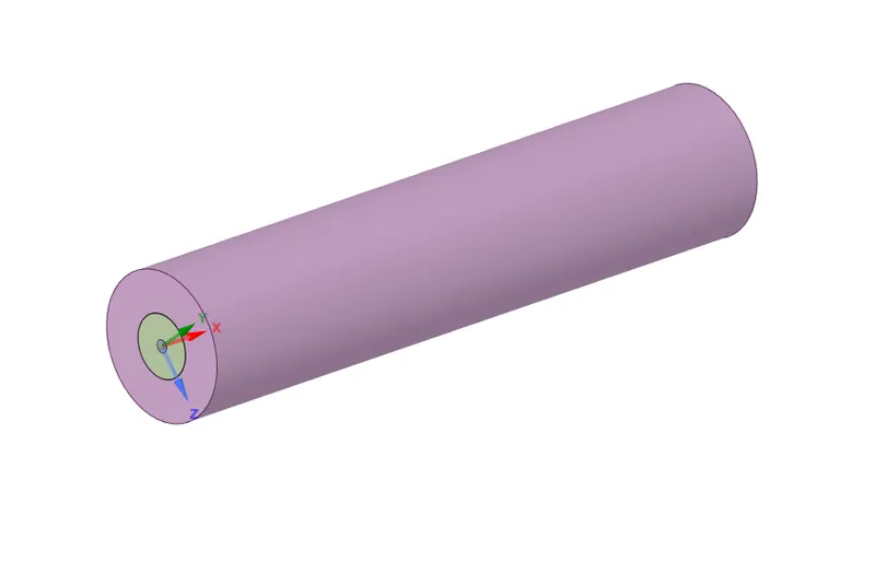
The domain in which the calculations needs to be carried out is extracted using Spaceclaim. The analysis is made axisymmetric for saving computational resources.

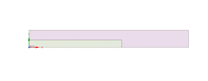
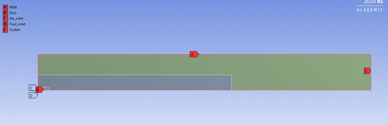
The geometry with named selection is shown below:

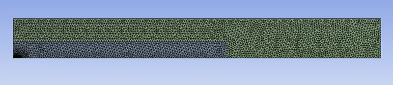
The mesh is shown below:

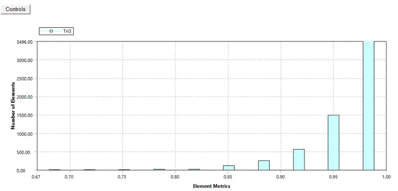
The mesh quality matrix is also given below:

SETUP OF THE SIMULATION

The simulation is set up as axisymmetric and a steady-state simulation with a pressure-based solver.

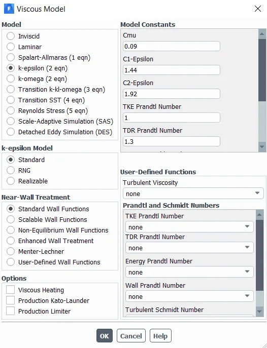
The turbulence model selected is the `k-epsilon` model.

The eddy dissipation model is used to model the species transport, and the setup of the species is shown below:

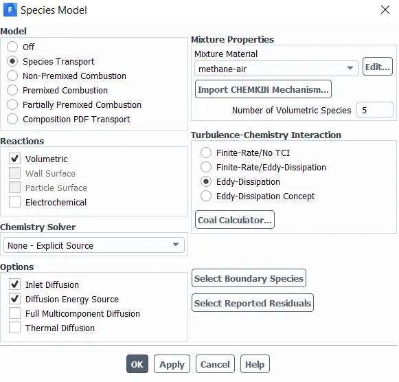
The methane-air mixture is selected and the mole fractions of the species can be adjusted in the boundary conditions. In the case where water needs to be added with the fuel, methane-air two-step needs to be selected for adding water. The models for `NO_x` and soot also needs to be turned on.

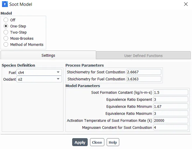
The soot model selected is one-step.

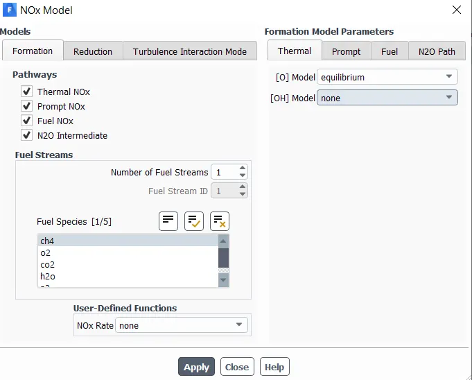
The model for `NO_x`is also selected as shown below:

The energy equation needs to be turned on.

The study is carried out in two parts, in the first section a simulation is run to calculate the mole fraction of different species at different axial locations. In the second part, water is added with the fuel to analyse its effect on the formation of soot and `NO_x`. The results are given in the next section.

RESULTS AND DISCUSSION

A simulation is run with the methane-air mixture to calculate the concentration of different species at different axial locations. Line probes are set at 0.1, 0.2, 0.3, 0.4 and 0.5 m axial locations on the combustor.

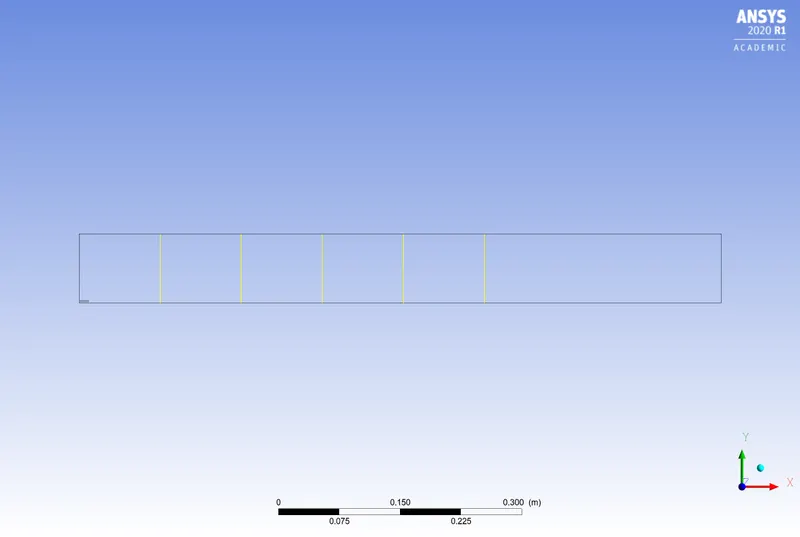
The mass fractions of different species at these locations are plotted using line plots and are shown below:

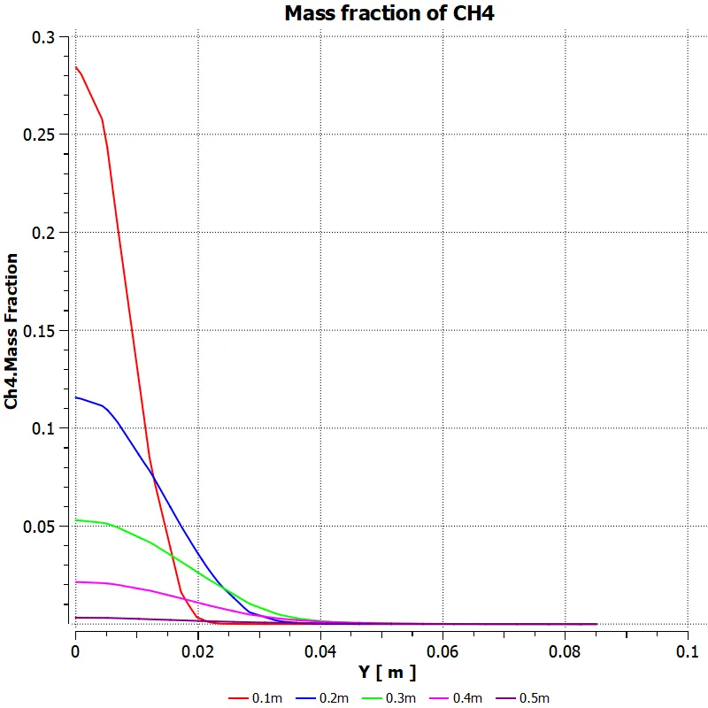
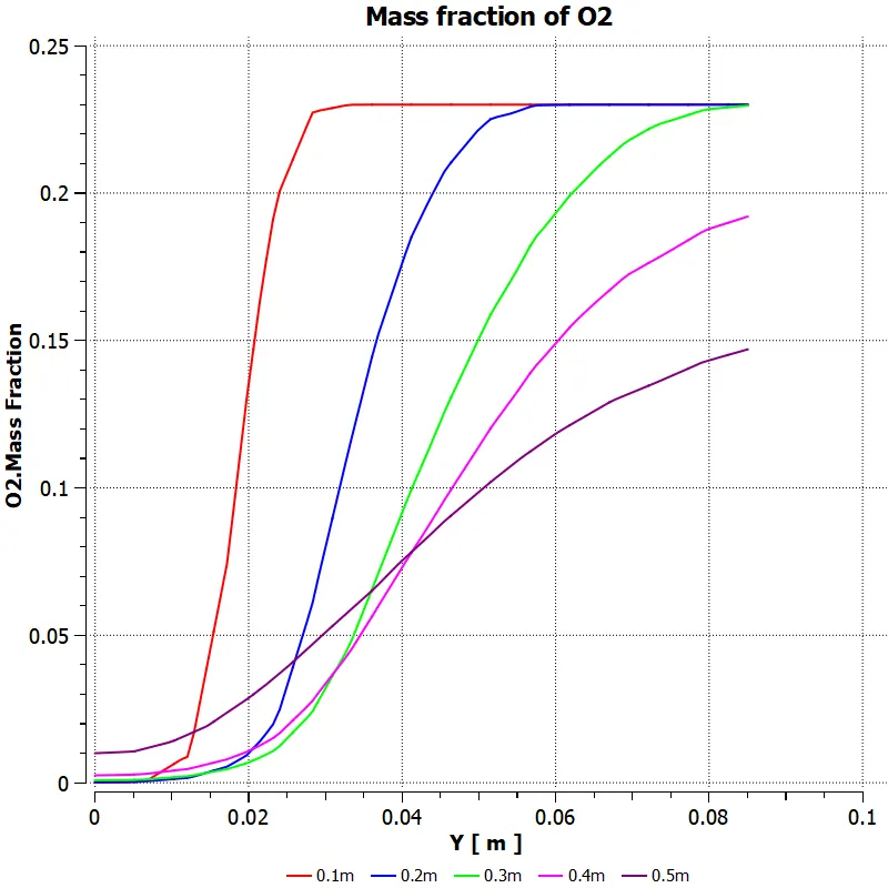
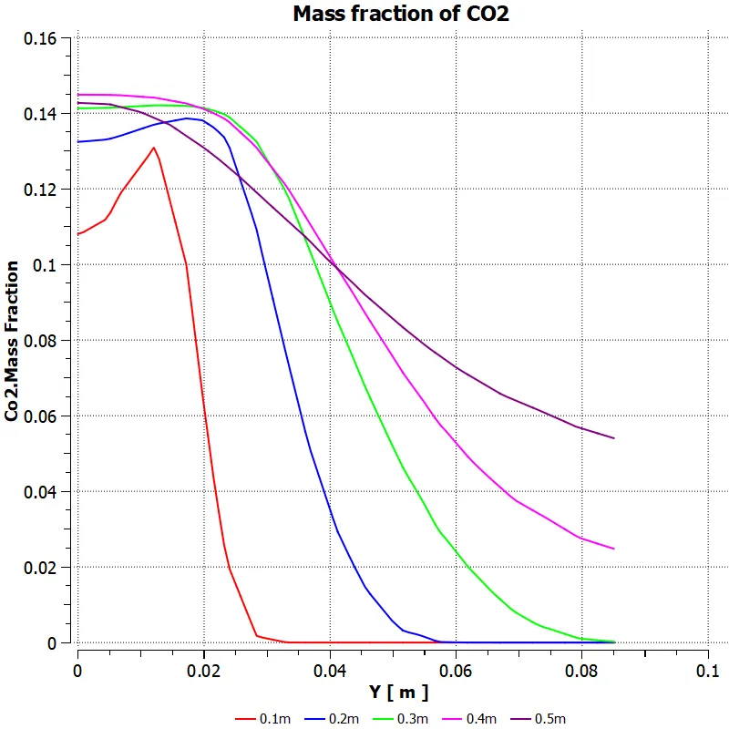
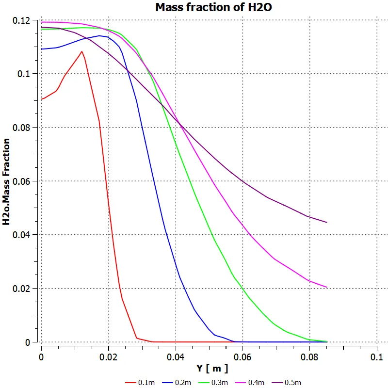
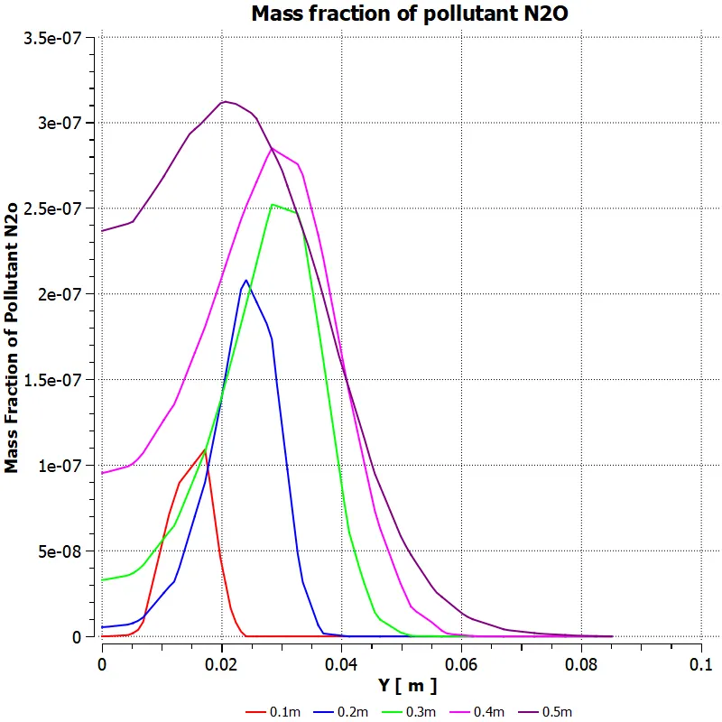
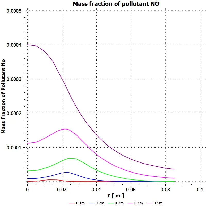
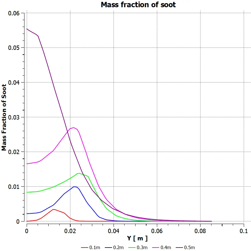
From the above plots, it can be seen that as the locations shifts away from the inlet of the combustor the concentration of fuel (`CH_4`) reduce and the case is same with that of oxygen also. For all the other species, the concentration increases as the axial location shifts away from the inlet. The maximum concentration of the pollutants are near the axis of the combustor and as the location moves towards the wall, the concentration of pollutants decreases. As the probe is moved away from the inlet we can see that the concentration of the pollutants also increases.

The temperature plots can be analysed to get a better picture. The temperature profile along the cross-section of the combustor is shown below:

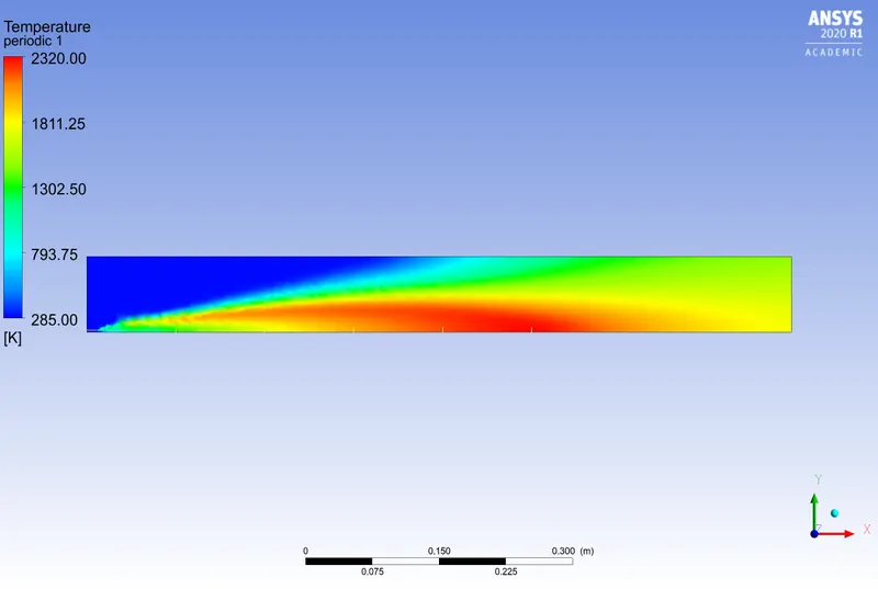
It can be seen that the more concentration of `NO_x`and soot is seen at regions of high temperature. It is important to note that as the temperature becomes higher the formation of pollutants also increases. One way to control the formation of these pollutants is by controlling the temperature.

In the second part of the study, water is added along with the fuel. The percentage of water is changed from 5% to 30% and an area-weighted average of the output temperature is monitored for each case. The mole fraction of water and methane is parameterised.

The parameter window is shown below:

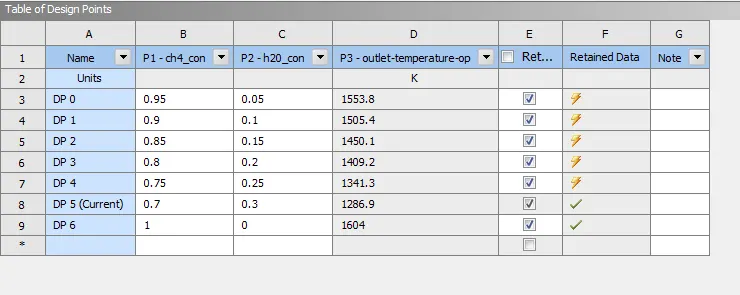
It can be seen that as the amount of water in the fuel is increased the temperature at the outlet is decreasing.

The temperature plot for 0% to 30 % water content is shown in the plots below:

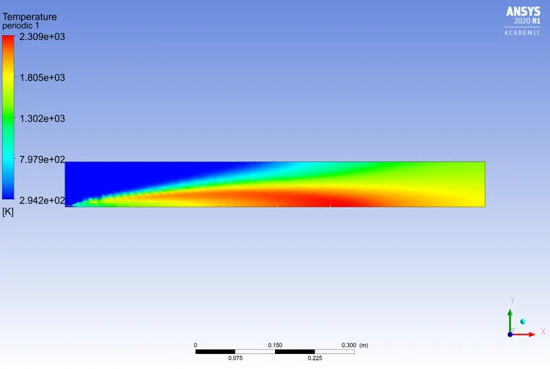
When there is no water added with the fuel the maximum temperature is 2309K, the water content is added which is 5% of the total mole fraction of the fuel, and the plot is shown below:

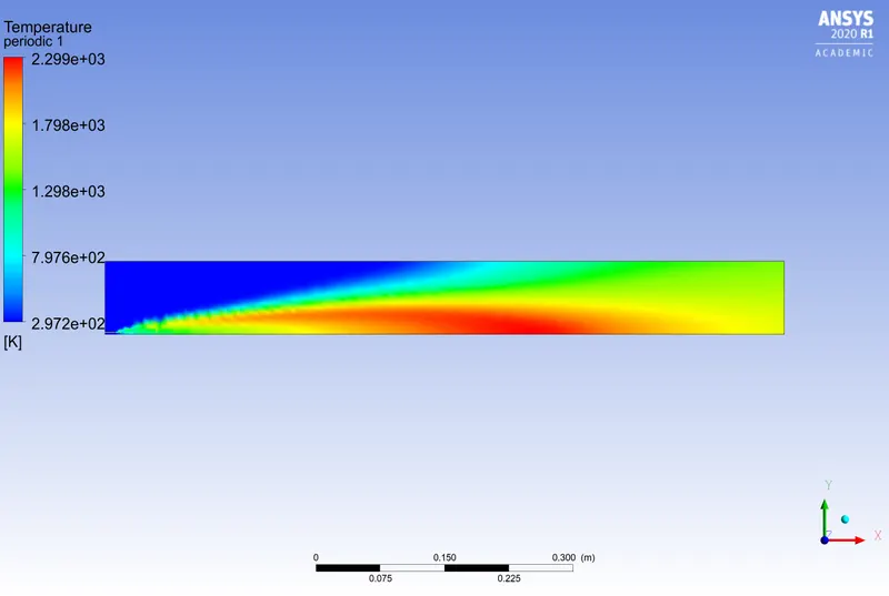
The maximum temperature, in this case, reduced to 2300 K, and as the water content is increased to 10% of the mole fraction of the fuel and the temperature plot is shown below:

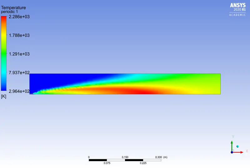
For a mole fraction of 15 % of the fuel the temperature plot is given below:

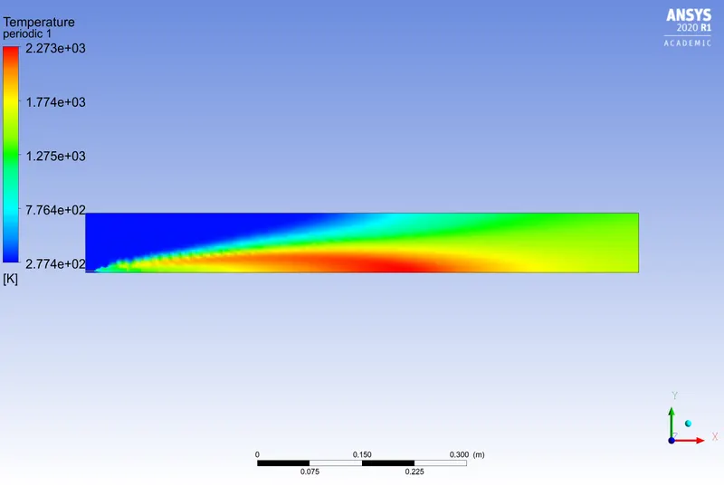
For a mole fraction of 20 % of the fuel the temperature plot is given below:

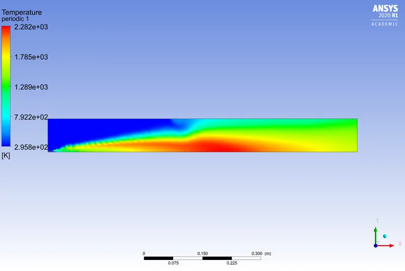
For a mole fraction of 25 % of the fuel the temperature plot is given below:

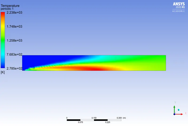
For a mole fraction of 30 % of the fuel the temperature plot is given below:

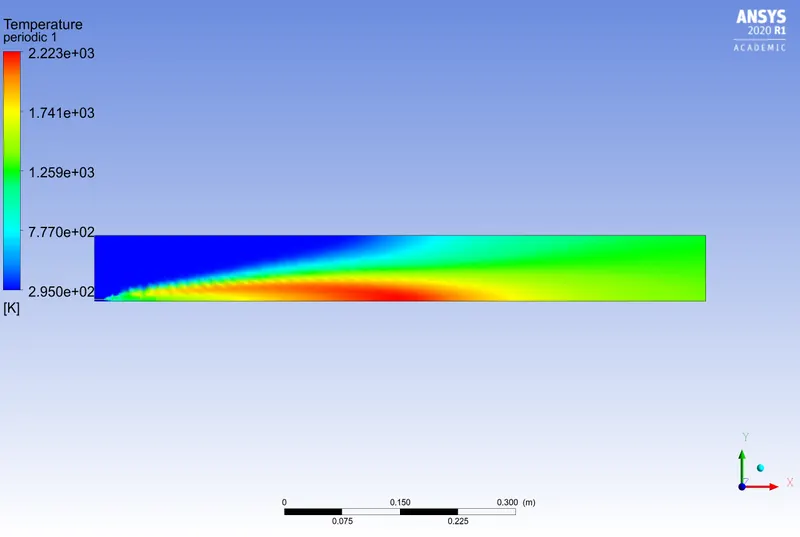
It can be seen that as the water content increases the temperature decreases as expected.

The contours of oxides of nitrogen and soot are given below. The contours of `N_2O` for 0% to 30% of mole fraction of water is shown in order.

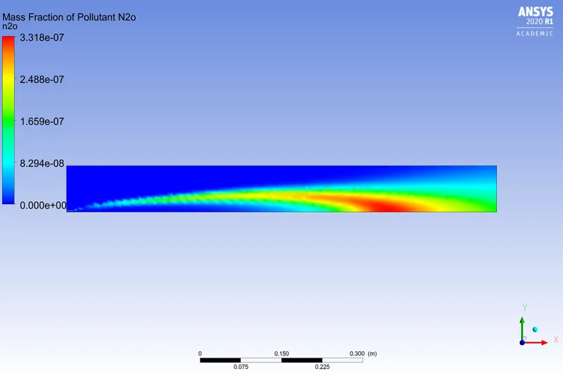
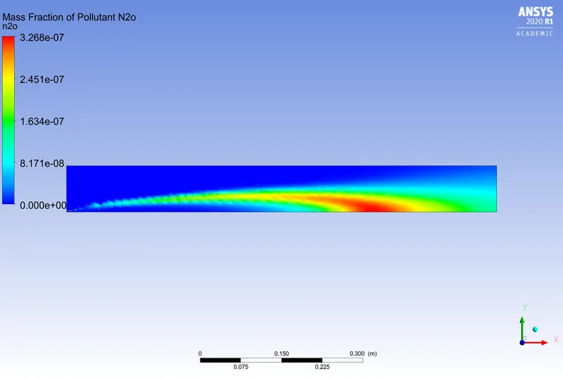
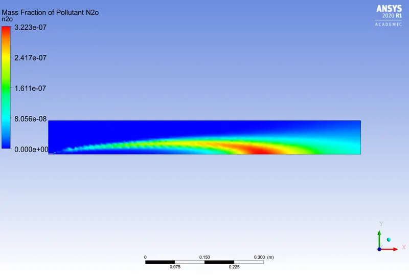
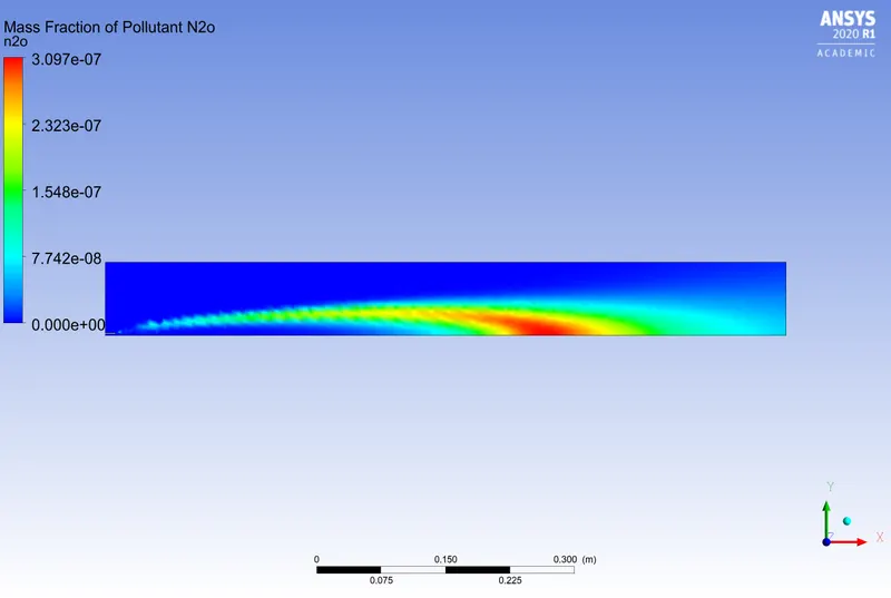
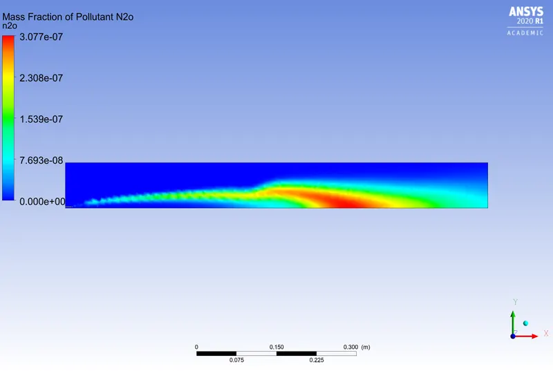
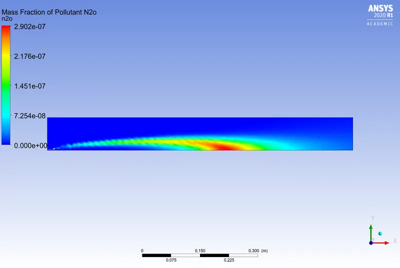
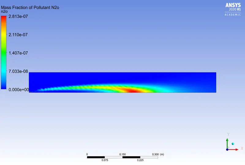
From the above images, it can be seen that as the content of water in the fuel increases, the temperature drops and also the concentration of `N_2O` formed also reduces. The same thing can be seen in the case of `NO` also. The contour plots of the same are given below in the order from 0% water to 30%.

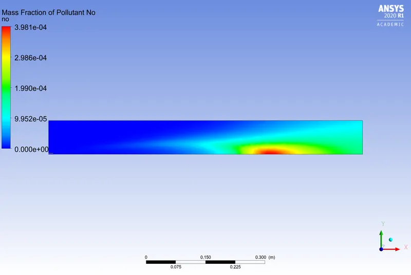
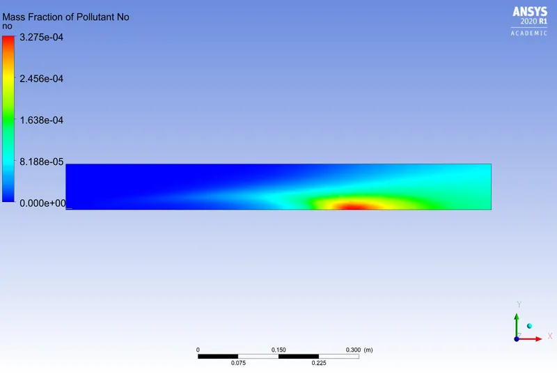
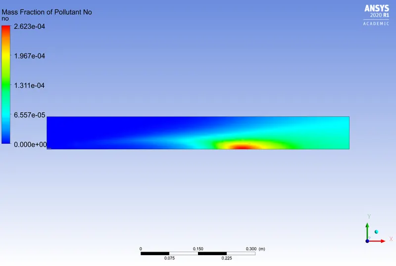
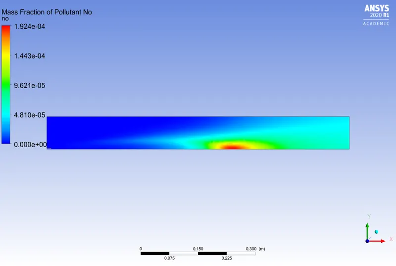
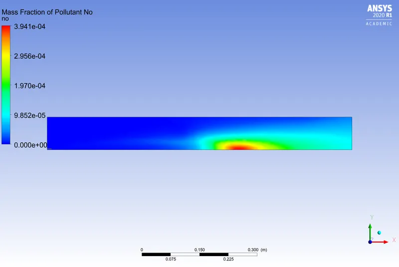
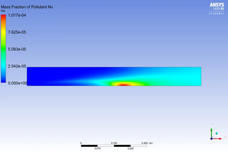
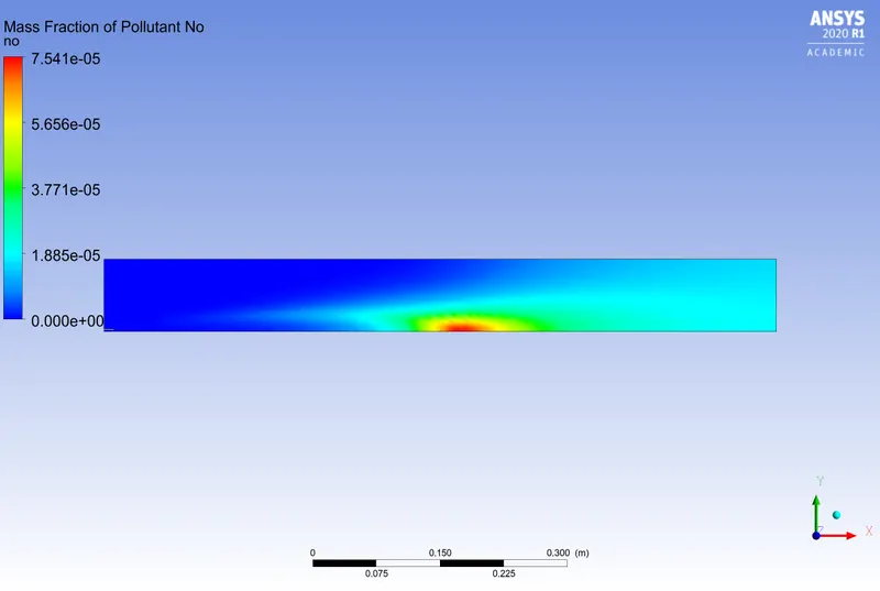
There is a large reduction in the formation of `NO` also as seen in the above images as the water content increases. The contour plots of soot formation for different mole fractions of water addition is given below:

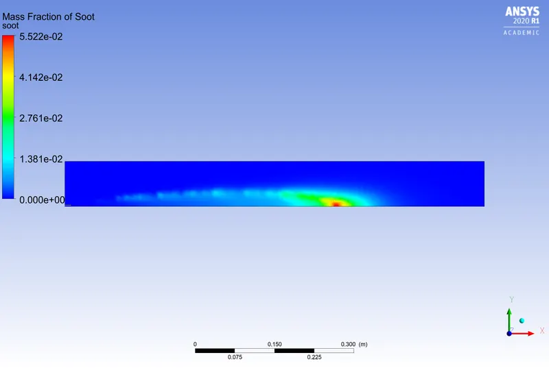
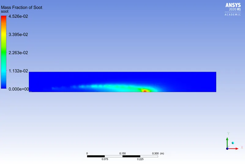
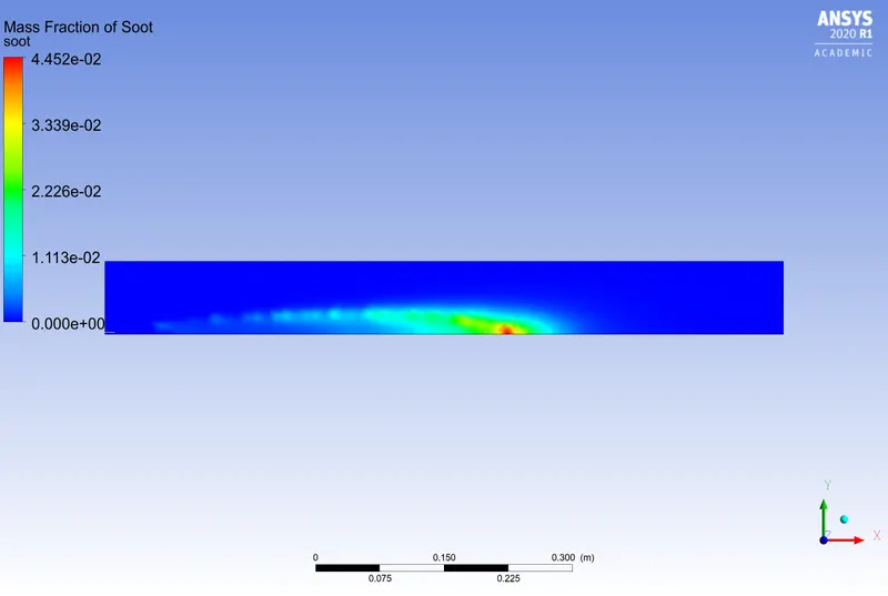
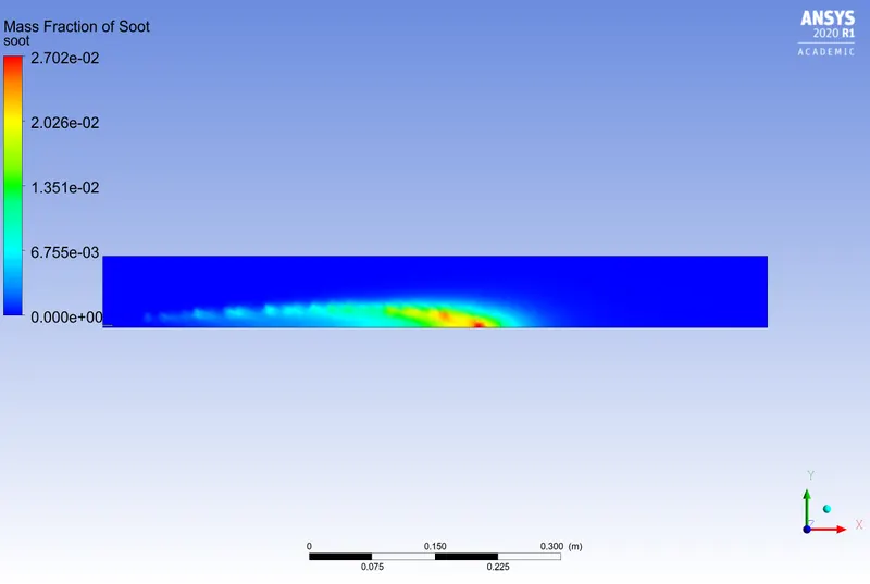
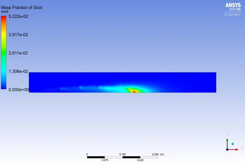
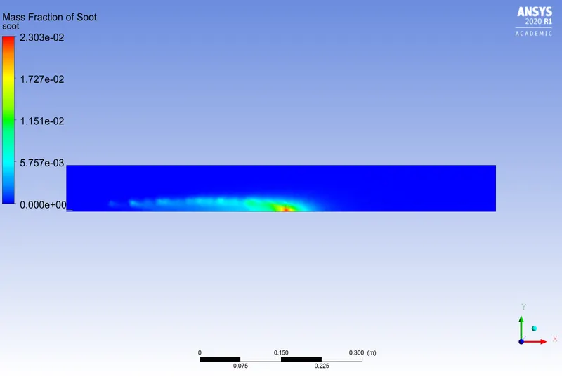
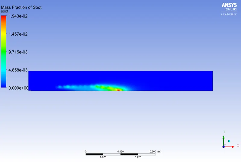
It can be seen that as the concentration of water in the fuel increases, the concentration of soot also decreases.

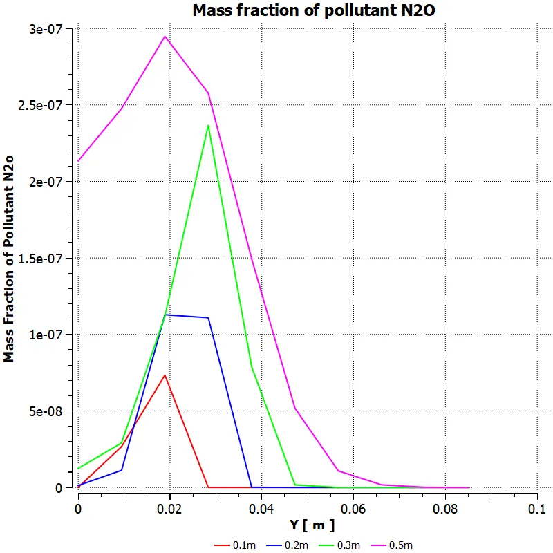
This can be also verified by using line plots at different axial locations. The mole fractions of soot and `NO_x` at the different axial location is shown in the following. The mole fraction of `N_2O` at different axial locations for different percentage of water is given below:

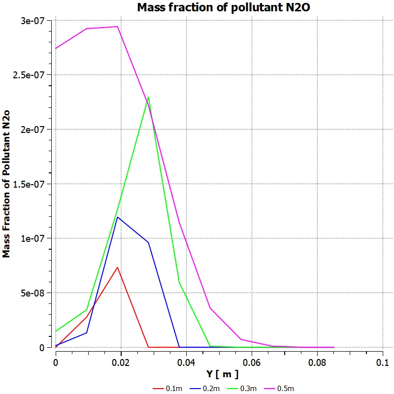
For mole fraction of water = 5% For mole fraction of water = 10%

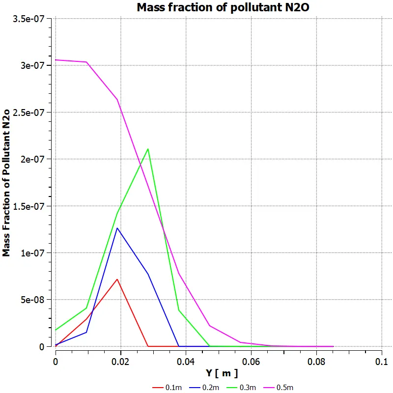
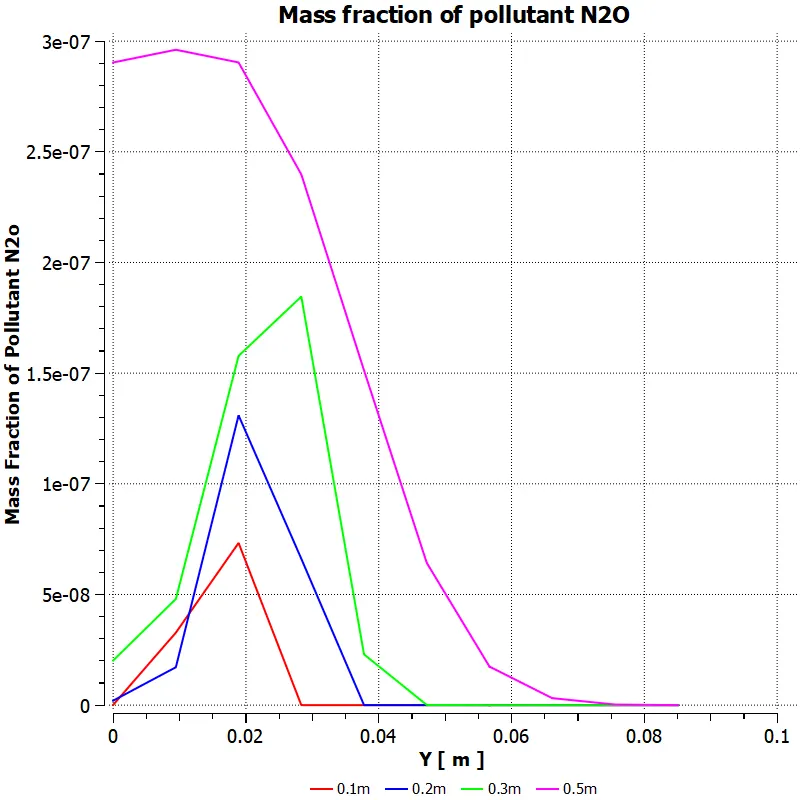
Mole fraction of water = 15% Mass fraction of water = 20%

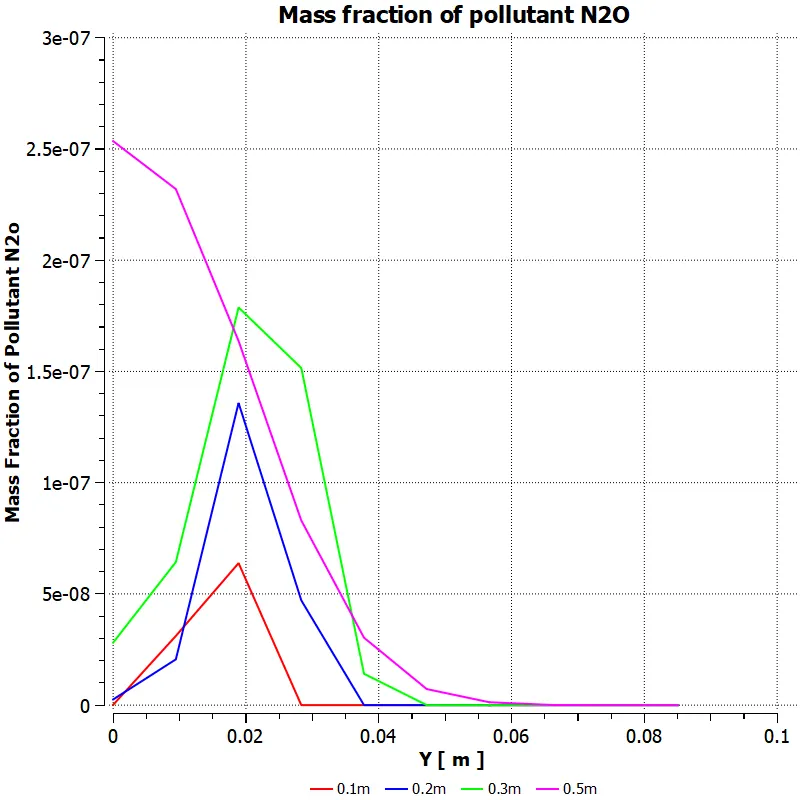
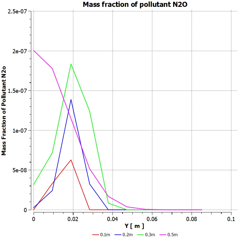
Mole fraction of water = 25% Mole fraction of water = 30%

From the line plots, it can be inferred that as the water content in the fuel increases, the concentration of `N_2O` formed reduces. The line plots depicting the concentration of `NO` is shown in the plots below:

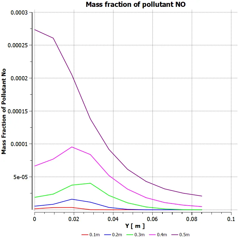
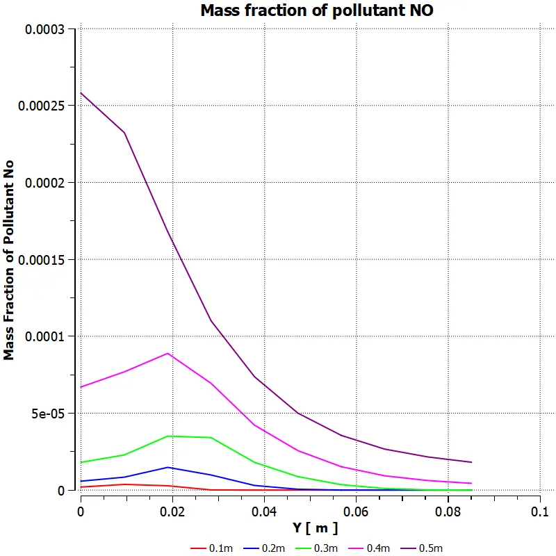
Mole fraction of water = 5% Mole fraction of water = 10%

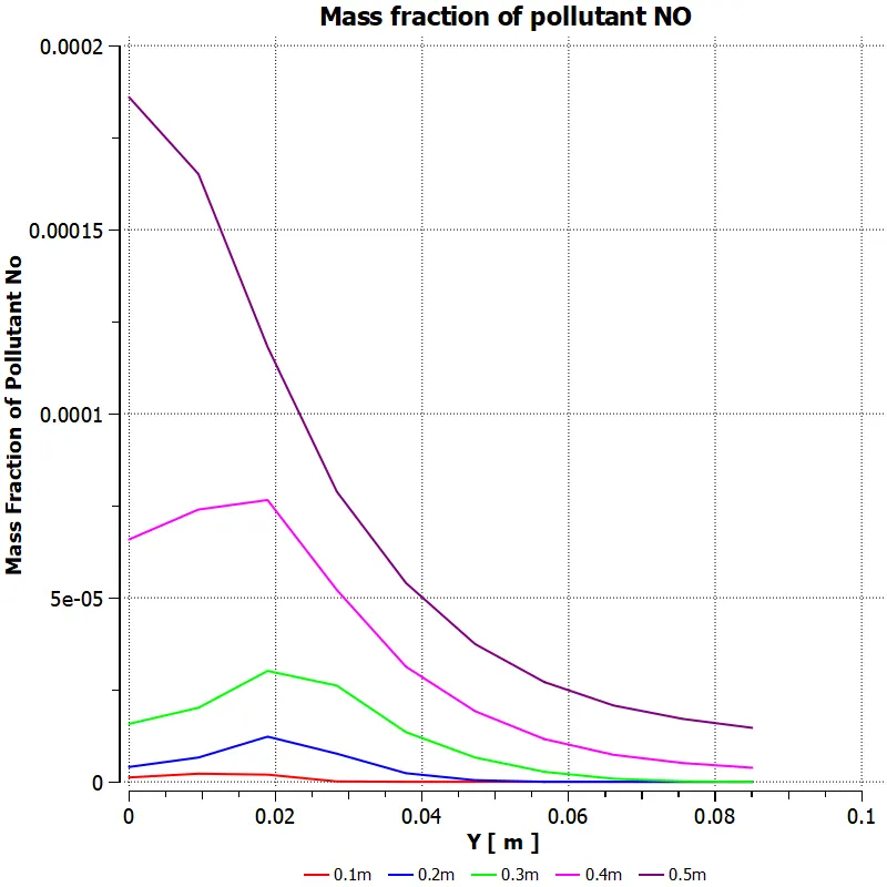
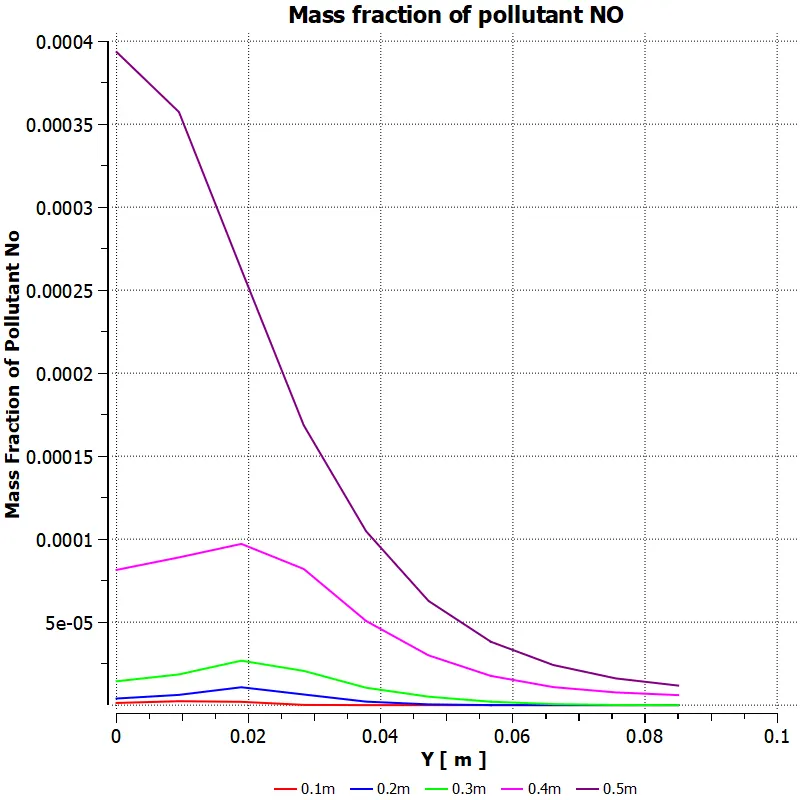
Mole fraction of water = 15% Mole fraction of water = 20%

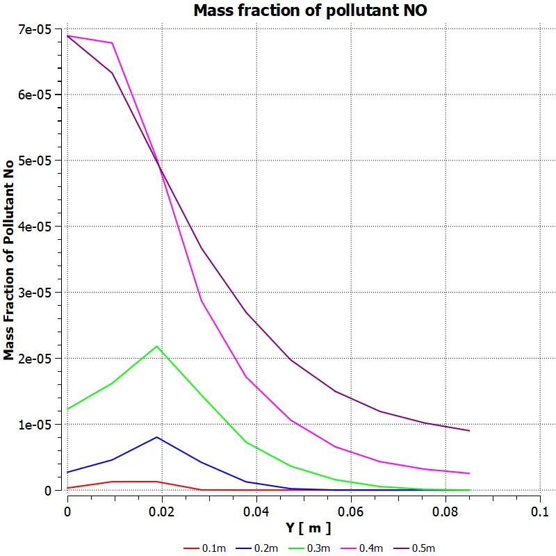
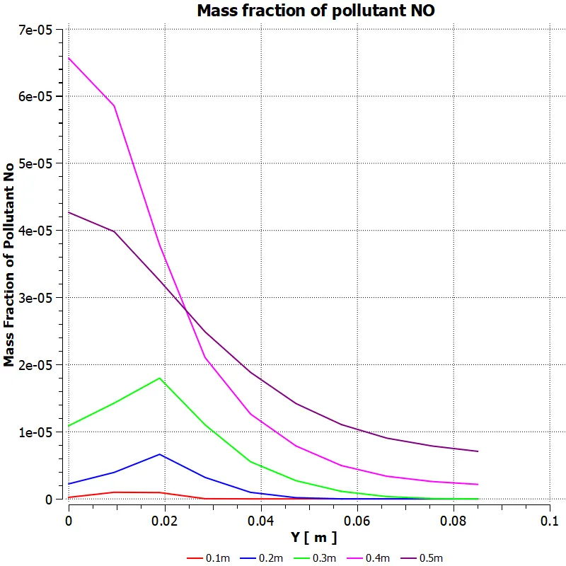
Mole fraction of water = 25% Mole fraction of water = 30%

The mass fraction of `NO` also decreases as the water added to the fuel is increased. The line charts for soot production at different locations along the axis is given below:

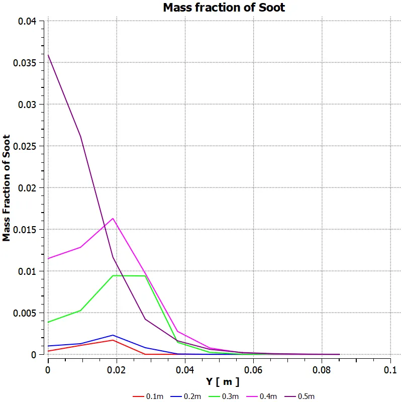
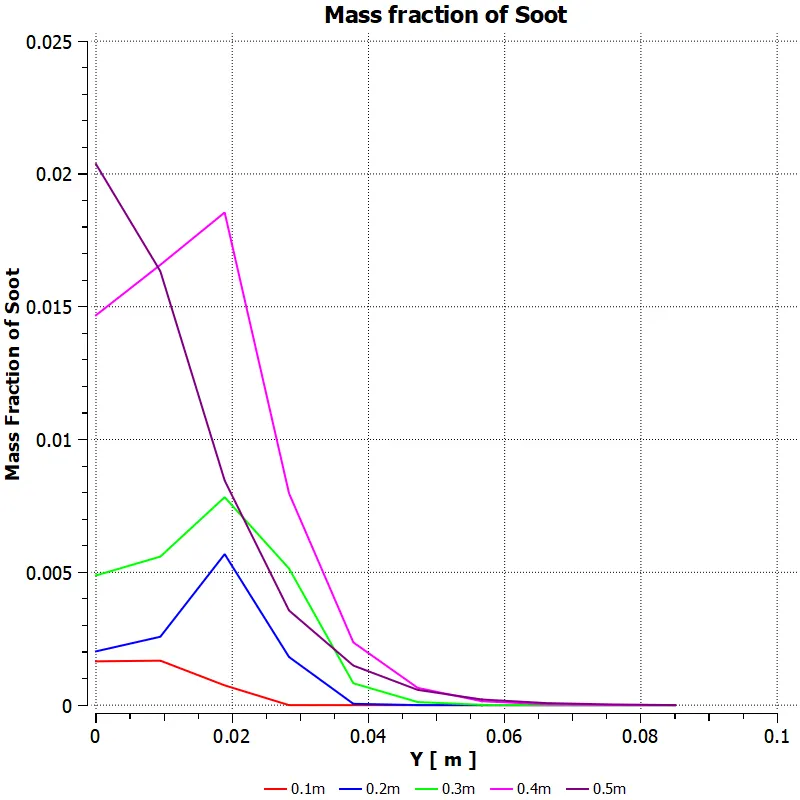
Mole fraction of water = 5% Mole fraction of water = 10%

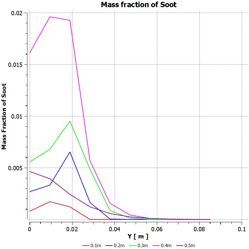
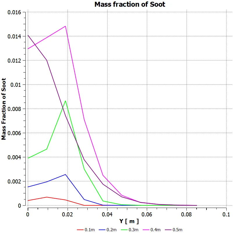
Mole fraction of water = 15% Mole fraction of water = 20%

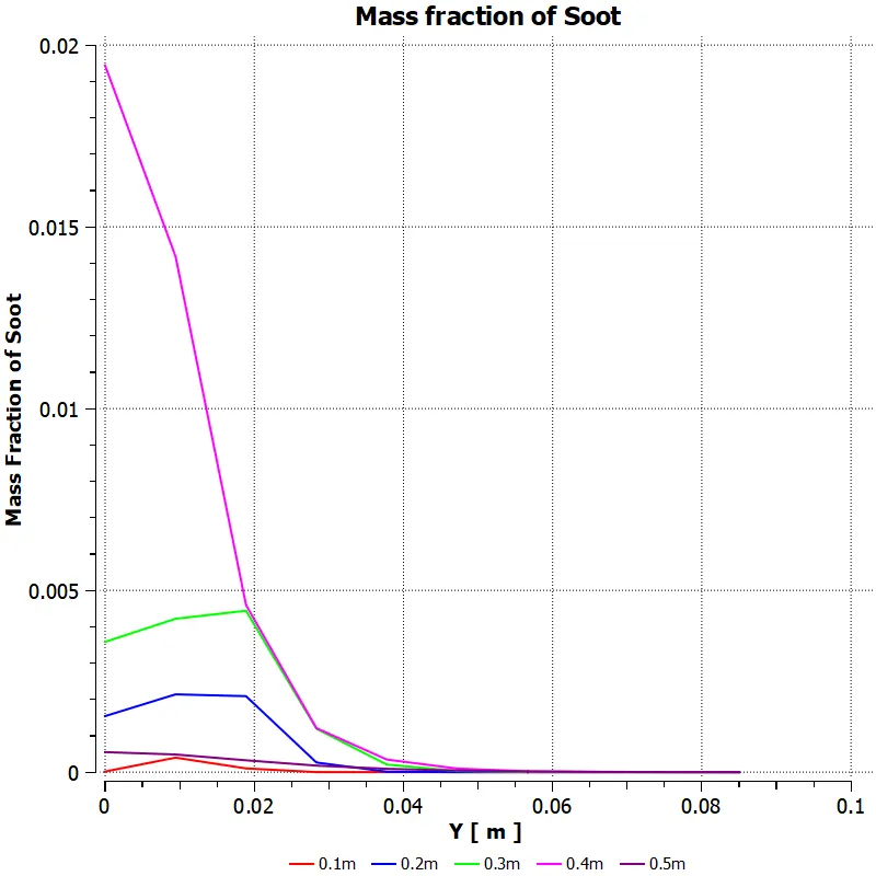
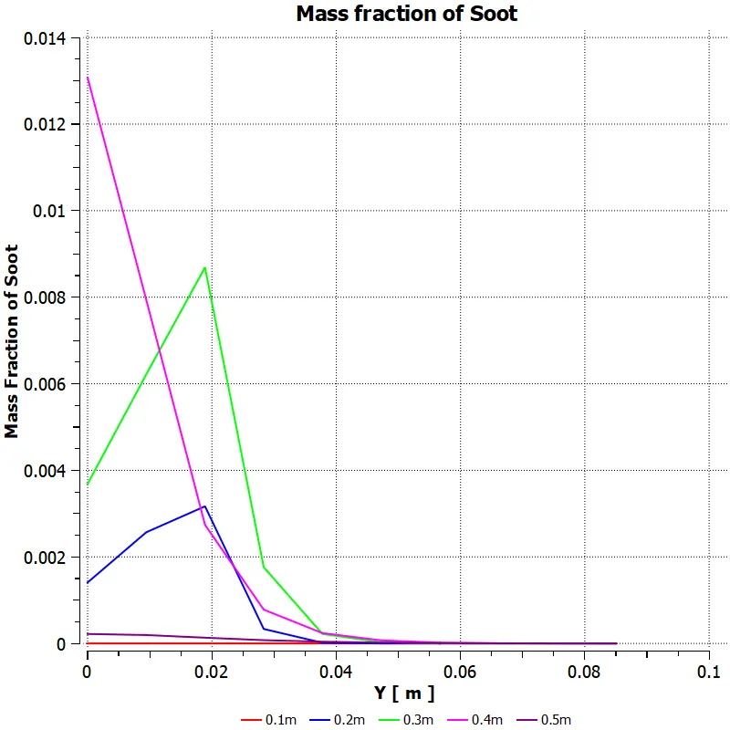
Mole fraction of water =25% Mole fraction of water = 30%

The production of soot also reduces as the water content in the fuel is increased. From the above results, it can be noted that the major contributor to `NO_x`pollution is `NO`. Low temperature doesn't favour the production of `NO`, when water is added to the mixture of fuel the otherwise stoichiometric mixture becomes lean which results in a reduced level of temperature generation which reduces the yield of `NO_x`. When the water is added the lean mixture becomes a source of less amount of hydrocarbon which in turn results in less production of soot. The lower temperature also is another reason for less production of soot.

This is also validated by using computer simulation. The contour plots and line plots also depict the same facts.

CONCLUSION

It is seen that as the water content in the fuel increases the temperature at the outlet decreases and also the maximum temperature also reduces. The nitrogen molecules which have high bond strength needs a higher temperature to form oxides. A lower temperature results in less yield of the oxides of nitrogen. This drop in temperature is achieved by using water along with the fuel.

As the water content in the fuel is increased the pollutant concentration reduces. The lean mixture and the reduction in the high temperature resulted in the reduction of pollutant concentration. It is also important to test different models for the prediction of the formation of soot and `NO_x`.

There was an anomalous behaviour while running the simulation at first when the simulation was run for more number of iterations the solution moved away from the converged solution or the solution overshoot happened. To avoid that a relaxation factor less than 1 was used or an under relaxation factor was used which eliminated the overshoot.

For an accurate prediction, we must first do a mesh independence test before carrying out the study due to the limitations of an academic licence it was not accurately done. By carrying out this study the concept of parametric study which was used in a previous challenge was successfully used which saved a lot of time. The parametric study in the latest version, ANSYS 2020 R2 had some bugs but it was perfect in ANSYS 2020 R1.

REFERENCE

http://citeseerx.ist.psu.edu/viewdoc/download?doi=10.1.1.193.290&rep=rep1&type=pdf

https://www.sciencedirect.com/science/article/pii/S1876610217337724

https://link.springer.com/article/10.1007/s00773-015-0303-8