Centrifugal Pump Design and Flow Simulation Analysis

AIM:

Design a centrifugal pump and perform the flow simulation of flow of a fluid using Solidworks Flow Simulation

OBJECTIVE:

To obtain a performance curve of a centrifugal pump, which is basically a plot of pressure ratio versus the mass flow rate of the pump at outlet in kg/s.

THEORY:

A centrifugal pump is a mechanical device designed to move a fluid by means of the transfer of rotational energy from one or more driven rotors, called impellers. Fluid enters the rapidly rotating impeller along its axis and is cast out by centrifugal force along its circumference through the impeller’s vane tips. The action of the impeller increases the fluid’s velocity and pressure and also directs it towards the pump outlet. The pump casing is specially designed to constrict the fluid from the pump inlet, direct it into the impeller and then slow and control the fluid before discharge.

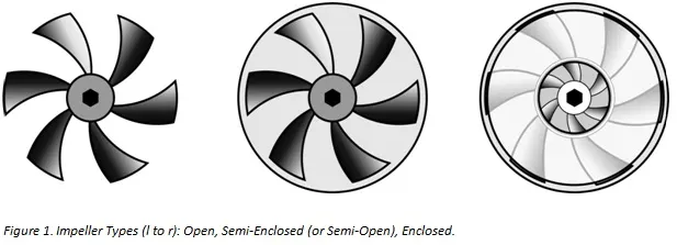
PROCEDURE:

1. Sketch the centrifugal pump and prepare the CAD model by taking suitable dimensions.

2. Enable Flow Simulation from the add-ins menu.

3. After that, the flow simulation wizard is used to set up all the parameters of the mathematical model.

4. Steps for wizard: (Note that rotation is checked, i.e. there is rotation of fluid involved in this study)

1. Give a suitable project name.
2. Select a proper unit system, preferably SI system.
3. Select a flow type. In our case, the flow of the fluid, i.e water, is through the inlet of the pump. Hence, it is an internal flow.
4. Select the proper fluid that is used in the simulation. Also, select the proper flow type, depending on the nature of the flow i.e laminar, turbulent or mixed.
5. Set wall conditions as it is. Do not make any changes as far as the challenge is considered.

5. Since this is an internal flow, the boundary conditions are needed to be set up. The typical boundary conditions used in this simulation are:

1. Environmental Pressure at inlet, equal to 1 bar, i.e 101625 Pa.
2. Velocity at outlet, initialed to a value of 15 m/s.

6. Check the computational domain after setting up the flow simulation. If the size of the domain is adequate, leave the size as it is.

7. The size of the mesh for this simulation was set to 4 due to hardware limitations of the laptop. Also make sure that the advanced channel refinement is selected.

8. Once the grid is selected, set the local surface goals. In our case, the main goal is to find out the mass flow rate at outlet, pressure at inlet and outlet respectively.

9. Finally, create the lids as the inlet and the outlet must be perfectly closed.

10. Run the simulation using parametric study as follows:

1. Select the input variable as the outlet velocity normal to the face of the outlet pipe. Enter the range of the velocity and the number of iterations for which the simulation must be run.

3. Select the output parameter as the main surface goal, i.e the mass flow rate, outlet pressure, inlet pressure, required cut plots and flow trajectories.

5. Check the scenario tab and run the simulation.

OBSERVATION AND RESULTS:

1. The outputs obtained after running the simulations are as follows:

Goal (Value)	Design Point 1	Design Point 2	Design Point 3	Design Point 4	Design Point 5	Design Point 6
Velocity normal to face (Outlet Velocity 1) [m/s]	17.5	20	22.5	25	27.5	30
SG Average Total Pressure 1 [Pa]	1242262.869	1194162	1043506.412	1057049.926	961090.8916	941725.0699
SG Average Total Pressure 2 [Pa]	101325	101325	101325	101325	101325	101325
SG Mass Flow Rate 1 [kg/s]	-2.290859864	-2.618377352	-2.945548997	-3.273002817	-3.59999635	-3.927454143

2. The cut plots obtained for oulet pressure for the 6 iterations are:

a. At 17.5 m/s

b. At 20 m/s

c. At 22.5 m/s

d. At 25 m/s

e. At 27.5 m/s

f. At 30 m/s

3. The flow trajecctories of the fluid particles is illustrated for the 1st iteration only.

Animation:

4. The performance curve of the pump was obtained, which is basically a plot of pressure ratio on the Y-axis and Mass flow rate of the fluid in kg/s on the X-axis.

5. The following graphs were also obtained after the simulation.

i. Mass flow rate

ii. Average total pressure at outlet

6. The plot data obtained after running the simulation is shown below:

SG Average Total Pressure 1 (Value)
	Design Point 1	Design Point 2	Design Point 3	Design Point 4	Design Point 5	Design Point 6
SG Average Total Pressure 1 [Pa]	1242262.869	1194162	1043506.412	1057049.926	961090.8916	941725.0699
SG Average Total Pressure 2 (Value)
	Design Point 1	Design Point 2	Design Point 3	Design Point 4	Design Point 5	Design Point 6
SG Average Total Pressure 2 [Pa]	101325	101325	101325	101325	101325	101325
SG Mass Flow Rate 1 (Value)
	Design Point 1	Design Point 2	Design Point 3	Design Point 4	Design Point 5	Design Point 6
SG Mass Flow Rate 1 [kg/s]	-2.290859864	-2.618377352	-2.945548997	-3.273002817	-3.59999635	-3.927454143

CONCLUSION:

1. From the results we can clearly see that the pressure is decreasing with the increase in velocity which is what was expected.

2. Along with this, we rate has a negative sign because mass is coming out of the system.

3. Also, we can observe from the flow trajectory that there is a significant loss due to eddy formtion which makes the outlet mass flow rate lesser than the inlet mass flow rate.