Study of performance curve on a Modeled Centrifugal Pump

Aim:

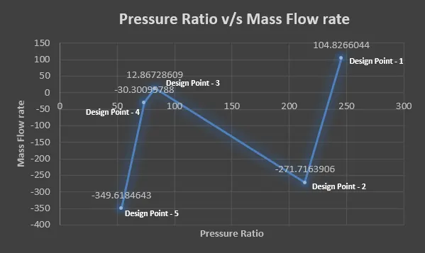
To study the performance curve on a modeled centrifugal pump and obtain a relationship between pressure ratio and mass flow rate.

Abstract:

In this study, a centrifugal pump is modeled with dimensions and studied for various pump performance characteristic parameters such as Fluid pressure, velocity, and turbulent energy inside the pump. These characteristics are studied by a parametric study generated while increasing outlet velocity from the range of 10m/s to 30m/s. Each case study gives the working condition of the pump which is later used to create the performance curves.

Theory:

Hydraulic machines that convert mechanical energy into hydraulic energy are called pumps.

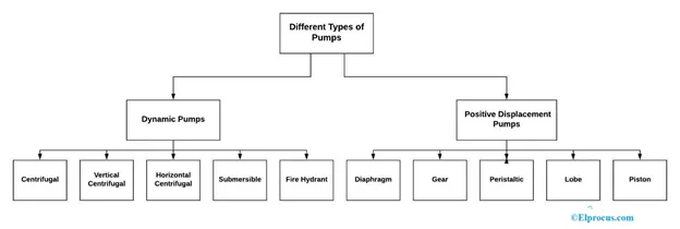
The hydraulic energy is in the form of pressure energy. If the mechanical energy is converted into pressure energy using centrifugal force acting on the fluid, the hydraulic machine is called the Centrifugal pump.

The centrifugal pump acts as a reverse of an inward radial flow reaction turbine. This means that the flow in centrifugal pumps is in the radial outward directions. The centrifugal pump works on the principle of forced vortex flow which means that when a certain mass of liquid is rotated by an external torque, the rise in pressure head of the rotating liquid takes place. The rise in pressure head at any point of the rotating liquid is proportional to the square of the tangential velocity of the liquid at that point (rise in pressure head = `frac{V^2}{2g}` or `frac{omega^2r^2}{2g}`. Thus, at the outlet of the impeller, where the radius is more, the rise in pressure head will be more and the liquid will be discharged at the outlet with a high-pressure head. Due to this high-pressure head, the liquid can be lifted to a high level.

Main Parts of a centrifugal pump:

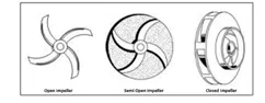
1. Impeller – The rotating part of a centrifugal pump is called an impeller. It consists of a series of backward curved vanes. The impeller is mounted on a shaft which is connected to the shaft of an electric motor.
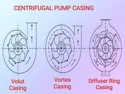
2. Casing – The casing of a centrifugal pump is similar to the casing of a reaction turbine. IT is an air-tight passage surrounding the impeller and is designed in such a way that the kinetic energy of the water discharged at the outlet of the impeller is converted into pressure energy before the water leaves the casing and enters the delivery pipe. The following three types of casings are commonly
3. Suction pipe with a foot valve and a strainer – A pipe with one end connected to the inlet of the pump and other end dipped in water sump is called the suction pipe. The foot valve opens only in an upward direction. A strainer is also fitted at the lower end of the suction pipe.
4. Delivery pipe – A pipe whose end is connected to the outlet of the pump and other end delivers the water at a required height as known as a delivery pipe.

A pump transfers mechanical energy from some external source to the liquid flowing through it and losses occur in any energy conversion process. The energy transferred is predicted by the Euler Equation. The energy transfer quantities are losses between fluid power and mechanical power of the impeller or runner. Thus, a centrifugal pump may be taken losses of energy. The kinds of loss of centrifugal pumps can be differentiated in internal losses and external or mechanical losses. The internal loss is hydraulic losses or blade losses by friction, variations of the effective area or changes of direction losses of quantity at the sealing places between the impeller and housing at the rotary shaft seals. The external or mechanical loss is sliding surface losses by bearing friction or seal friction [2]

Terminologies:

• Suction Head(h_s) – It is the vertical height of the centerline of the centrifugal pump above the water surface in the tank or pump from which water is to be lifted. This height is also called suction lift and is denoted by ‘h_s’.
• Delivery Head(h_d) – The vertical distance between the centerline of the pump and the water surface in the tank to which water is delivered is known as delivery head. This is denoted by ‘h_d’
• Static Head (H_s) ­– The sum of suction head and the delivery head is known as static head. This is represented by ‘H_s’ and is written as H_s=h_s + h_d
• Manometric head (H_m) – The manometric head is defined as the head against which is a centrifugal pump has to work. It is denoted by ‘H_m’

`H_m = h_s+h_d+h_fs+h_fd+frac{(V_d)^2}{2g} = frac{(V_w2)*(u_2)}{g}`

V_d = Velocity of water in the delivery pipe

h_fs = frictional head loss in the suction pipe

h_fd = frictional head loss in the delivery pipe

• Efficiencies of Centrifugal Pump

Manometric Efficiency – Ratio of the manometric head to the head imparted by the impeller to the water is known as manometric efficiency `eta_man =`(Manometric Head)/(Head imparted by the impeller to water`

Mechanical efficiency – The power at the shaft of the centrifugal pump is more than the power available at the impeller of the pump. The ratio of the power available at the impeller to the power at the shaft of the centrifugal pump is known as mechanical efficiency. `eta_m =`(Power at the impeller)/(Power at the shaft)

Overall efficiency – Defined as the ratio of the power output of the pump to the power input to the pump. The power output of the pump in KW. `eta_o = eta_man*eta_m`

Design Formulae and Considerations

• Minimum speed for starting a centrifugal pump – If the pressure rise in the impeller is more than or equal to the manometric head (H_m), the centrifugal pump will start delivering water. Otherwise, the pump will not discharge any water, though the impeller is rotating. When the impeller is rotating, the water in contact with the impeller is also rotating. This is the case of a forced vortex. `N = frac{120*(eta_man)*(V_w2)*D_2}{pi[(D_2)^2-(D_1)^2]}`
• Specific Speed of Centrifugal Pump (N_s) – Specific speed of a centrifugal pump is defined as the speed of geometrically similar pump which would deliver 1m³/s against a head of 1m. It is denoted by ‘N_s’ `N_s = frac{N*sqrtQ}{(H_m)^(3/4)}`
• Power of the pump – `P = frac{rho*g*Q*H_m}{75}`
• Discharge – [Q = Area * Velocity of flow]
  • `Q = pi*D_1*B_1*V_f1 = pi*D_2*B_2*V_f2`

B₁ and B₂ width of the impeller at inlet and outlet

V_f1 and V_f2 velocities of flow at inlet and outlet.

Objective: To demonstrate the effects of increasing Outlet velocity on fluid pressure, discharge, and turbulence inside a centrifugal pump.

Design Modeling Setup:

1. Sketch a circle of diameter – 300mm
2. Use the curves tool and select the sketched Circle. With Start revolution angle at 100 degrees.
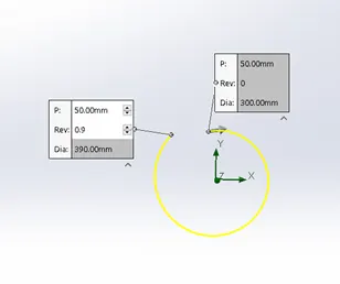
3. Create two planes such that both the planes are at the endpoints of this helix.
4. Draw two circles on these recently created planes such that the center of the circle is pierced by the helical curve. With the diameter of both the circle being 150mm and 50mm.
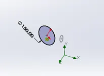
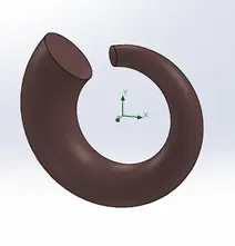
5. Now use the loft tool to create the main volute casing of the Centrifugal pump.
6. Now sketch a line extending in the Y-axis of length 450mm.
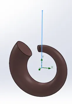
7. Create a plane at the endpoint of this line. Sketch a circle of diameter 200mm.
8. Now connect the endpoint of line and center of larger circle diameter 150mm with a spline such that this spline is tangent to the extended Y-axis line and is tangent to the helical curve also.
9. Use the loft tool to have the outlet of the centrifugal pump using the spline as the centerline guide.
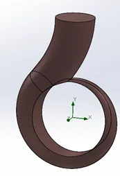
10. Make an extruded cut of diameter – 330mm. The model would resemble something like this
11. Sketch a circle of 345mm diameter. Now Use extrude boss/base midplane and extend it till 240mm
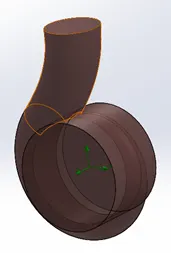
12. Use cut loft to create a hollow section at the upper end of the outlet pipe. By selecting entities and converting entities at the exit and the circle of 150mm diameter and creating an offset that entity at 3mm inside. Now use Cut loft and select these new offset entities and using end spline as the centerline guide.
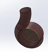
13. Cut an extruded cut of diameter 330mm from the center of the circle.
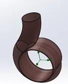
14. Now convert the entity of circle – 50mm and offset this entity at 3mm inside. Cut loft to have hollow volute casing from the smaller circle to the larger circle diameter – 150mm offset of 3mm. With the centerline guide being the helical curve.
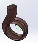
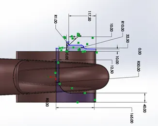
15. Now sketch as shown in the figure below. This will create the base and impeller eye diameter after using revolve boss/base. The end result would like this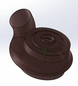
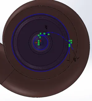
16. Now sketch the impeller inlet and outlet diameter along with the blade inlet and outlet angle as shown
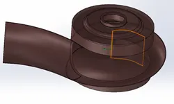
17. Now draw a circle of blade thickness and draw offset of the line that joins inlet impeller diameter to outlet impeller diameter equal to this blade thickness.
18. Extrude this body and it would resemble a single semi-closed vane.
19. Use a circular pattern to have 8 blades in this centrifugal pump.
20. Now extrude boss/base a circular sketch for the blade’s base plate such that it covers all the vanes in the domain and doesn’t touch the volute casing. This would be used in the simulation setup.
21. Create lids at the inlet and outlet of the pump to make it a water-tight model ready for the flow simulations.

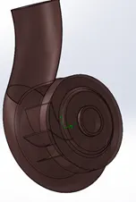
Simulation Setup:

1. Setup a flow wizard with internal flow simulations and check the boxes of gravity and rotations with Local regions (Averaging). Use fluid as water
2. Now go to the Input data -> Component control. Uncheck the boss extrude done at STEP – 20 in Design Modeling setup.
3. Add rotating region of the same Boss extrudes of STEP – 20 with a rotation of 1000rad/s.
4. Add boundary conditions of Environment pressure at inlet lid and Outlet velocity – 10m/s at the outlet lid.
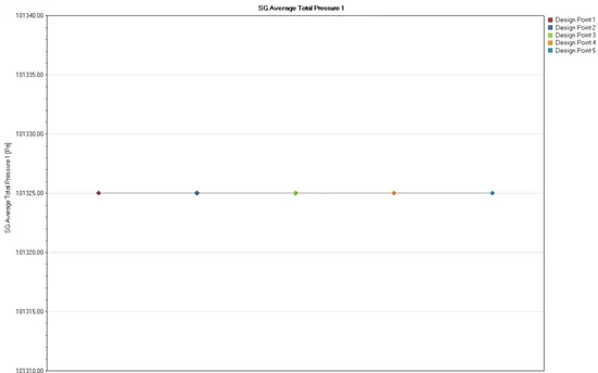
5. Setup surface goals of Total Average pressure at inlet and outlet lids and Global goals of Mass flow rate. Add Equation goals of [Pressure ratio – Total Pressure Outlet/ Total Pressure inlet]. [Discharge – Outlet area*Outlet velocity (Q = A*V)]
6. Change global meshing refinement to level – 5 and local mesh of Boss-Extrude STEP – 20 and inside surface of the volute casing to refinement level – 3.
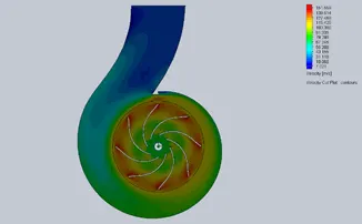
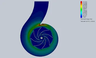
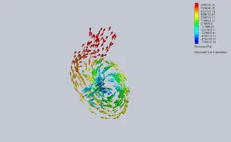
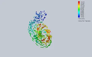
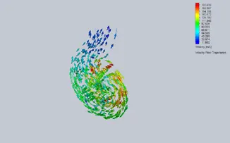
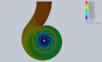
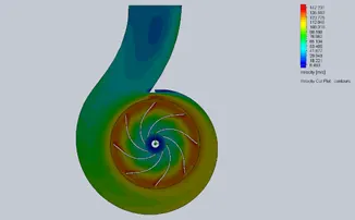
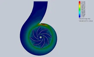
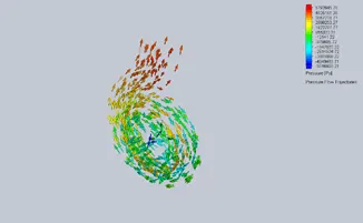
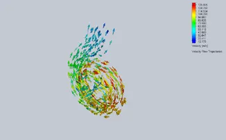
7. Now add Pressure Cut-plots, Velocity Cut-plots, and Turbulent Energy Cut-plots. Alon with Pressure flow trajectories and Velocity flow trajectories.
8. Now go to Input Data -> Calculations controls option to uncheck all the boxes in the finishing tab except iterations and change it to 700 iterations.
9. Now set up a parametric study with the boundary conditions of Outlet velocity being the input parameters and tick all the goals, flow trajectories, and cut-plots as the Output parameters.

Results & Analysis:

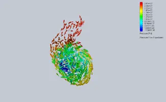
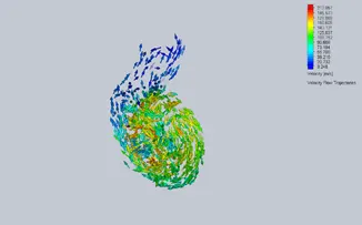
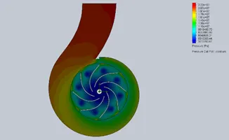
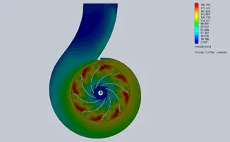
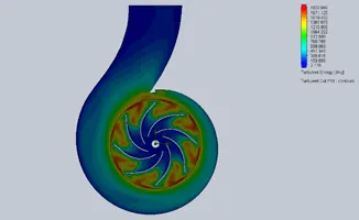
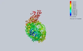
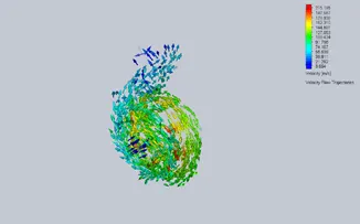
Case – 1: When Outlet velocity – 10m/s.

Pressure Cut-Plot	Velocity Cut-Plot
Turbulent Energy Cut-Plot
Pressure Flow Trajectory	Velocity Flow Trajectory

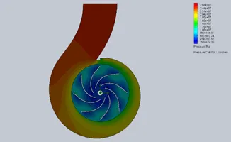
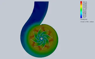
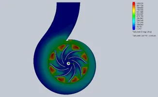
Case – 2: When Outlet velocity – 15m/s.

Pressure Cut-Plot	Velocity Cut-Plot
Turbulent Energy Cut-Plot
Pressure Flow Trajectory	Velocity Flow Trajectory

Case – 3: When Outlet velocity – 20m/s.

Pressure Cut-Plot	Velocity Cut-Plot
Turbulent Energy Cut-Plot
Pressure Flow Trajectory	Velocity Flow Trajectory

Case – 4: When Outlet velocity – 25m/s.

Pressure Cut-Plot	Velocity Cut-Plot
Turbulent Energy Cut-Plot
Pressure Flow Trajectory	Velocity Flow Trajectory

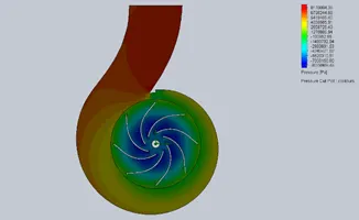
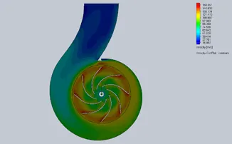
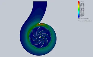
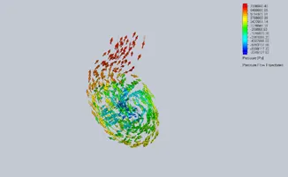
Case – 5: When Outlet velocity – 30m/s.

Pressure Cut-Plot	Velocity Cut-Plot
Turbulent Energy Cut-Plot
Pressure Flow Trajectory	Velocity Flow Trajectory

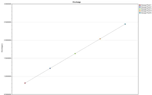
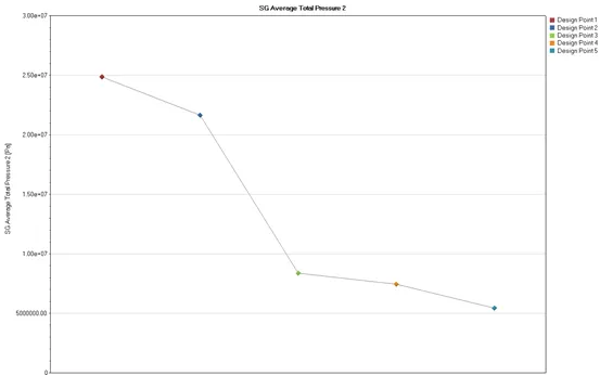
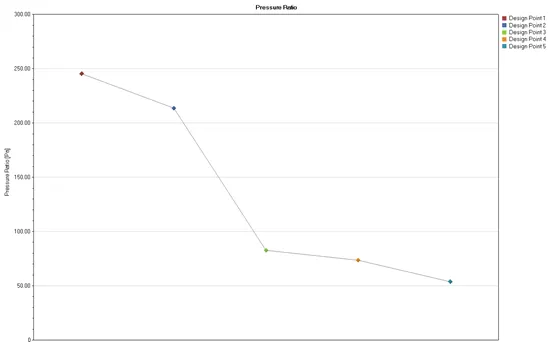
The goal results after the parametric study are as follows

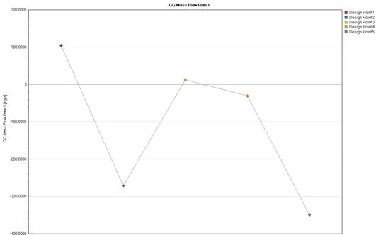
Conclusion:

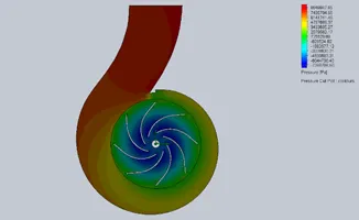
It can be clearly seen from the pressure plots that there is a low-pressure region created at the leading edge of the blade and also at low outlet velocity even at the back-end of trailing edge of the blade of modeled pump, this creates the favorable condition for the pump to suck the fluid inside. Lower pressure in the fluid is seen inside the volute areas with a narrower path compared to the wider discharge tube. Due to this low pressure in these areas, the velocity cut-plot shows that the fluid velocity is higher in such areas as compared to discharge tube areas. Interestingly the fluid velocity is seen highest in the trailing edge of the blade at all outlet velocities. This is due to a lot of water recirculation in the area which would account for pump efficiency losses which can be reduced by changing the outlet blade angle in the modeled pump. The turbulent energy seen at low velocities in the vicinity of the trailing edges of the blade is also taken into account during analysis.

The discharge of the pump is a function of the Outlet area and Outlet Velocity. This study conforms with the following statement as there is a steady rise in discharge with increasing outlet velocity. With increasing outlet velocity, the outlet pressure (SG Avg total pressure – 2) is decreasing and hence the pressure ratio is also seen decreasing. In the end there is a graph plotted between the pressure ratio v/s mass flow rate.

References

[1]	D. R. Bansal, A Textbook of fluid mechanics and Hydraulic machines, Laxmi Publication Ltd..
[2]	S.Chakraborty and K.M.Pandey, "Numerical Studies on Effects of Blade Number Variations on Performance of Centrifugal Pumps at 4000 RPM," International Journal of Engineering and Technology, Vols. Vol.3, No.4, August 2011.
[3]	K. C. Thin, M. M. Khaing and K. M. Aye, "Design and Performance Analysis of Centrifugal," World Academy of Science, Engineering and Technology.