Bode Plot and Step Response

OBJECTIVE:

• To explain the Matlab commands related to the Transfer function, pole-zero-gain, and step response. with an example apply the commands in the Matlab.
• For the unity feedback system shown in the figure below:

• Determine the closed-loop step response using MATLAB commands.
• To Explain the MATLAB model ‘scdspeedctrl’. Comment on results for non-tuned PID gain values.
• To explain the importance of the bode plot for control system design and Using MATLAB makes a bode plot of a transfer function.

TRANSFER FUNCTION:

• Transfer Functions are Frequency domain representation of linear time-invariant systems.
• Consider a continuous-time SISO dynamic system represented by the transfer function sys(s)=N(s)/D(s), where s=j`omega` and N(s) and D(s) are called the numerator and denominator polynomials.
• The tf model object can represent SISO or MIMO transfer functions in continuous time or discrete-time.
• Using tf command in Matlab to create real-valued or complex-valued transfer function models or to convert the dynamic system models to transform function form.

The following list contains a representative subset of the functions you can use with tf models. In general, any function applicable to Dynamic system models is applicable to tf object.

• Linear analysis.
• Stability analysis.
• Model Transformation.
• Model Interconnection.
• Controller design.

Linear Analysis:

step	Step response plot of the dynamic system; step response data
impulse	impulse response plot of the dynamic system; impulse response data
1sim	Plot simulated time response of the dynamic system to arbitrary inputs; simulated response data.
bode	Bode plot of frequency response or magnitude and phase data.
nyquist	Nyquist plot of the frequency response
nichols	Nichols chart of the frequency response
bandwidth	Frequency response bandwidth

Stability Analysis:

pole	Poles of the dynamic system
zero	Zeros and gain of SISO dynamic system
pzplot	Pole-Zero plot of dynamic system model with plot customization options
margin	Gain margin, phase margin, and crossover frequencies.

Model Transformation:

zpk	Zero-Pole gain model
ss	State-space model
c2d	convert the model from continuous to discrete-time
d2c	convert the model from discrete to continuous-time
d2d	Resample discrete-time model.

Model Interconnection:

feedback	Feedback connection of multiple models
connect	Block diagram interconnections of dynamic systems
series	Series connection of two models
parallel	parallel connection of two models

Controller Design:

pidtune	PID tuning algorithm for the linear plant model
rlocus	Root locus plot of the dynamic system
lqr	Linear-Quadratic Regulator(LQR) design
lqg	Linear-Quadratic Gaussian(LQG) design
lqi	Linear Quadratic Integral Control
kalman	Kalman filter design, Kalman estimator

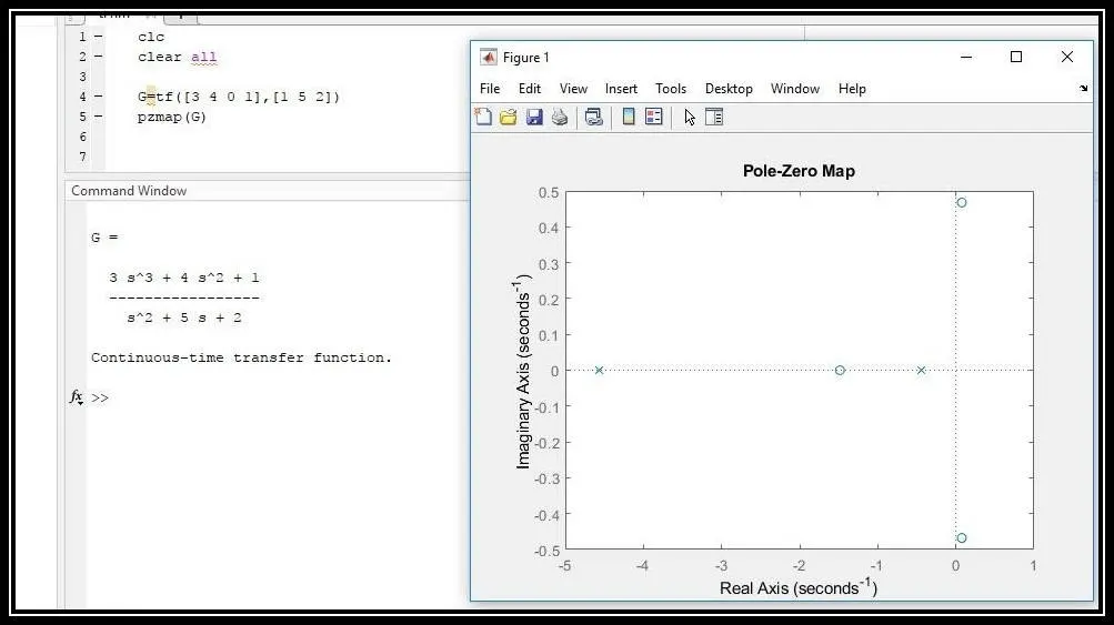
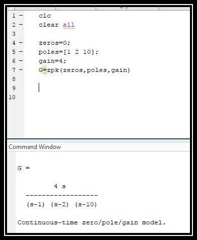
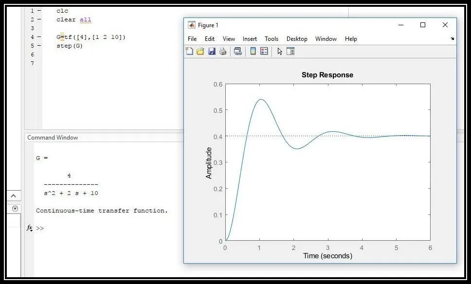
Some of the commands used in the Matlab program as follows:

2)

In the first step, the equation is rearranged and the coefficients are taken for the transfer function representation.

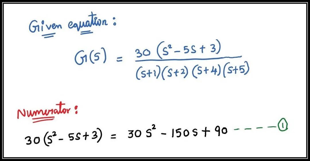
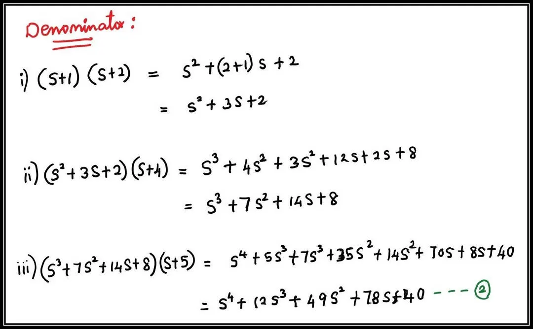
• The coefficients of S are taken in the descending Power of S and it used in tf command in Matlab.

Without Feedback :

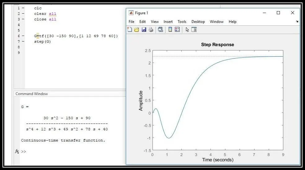
Result:

1)Peak response:

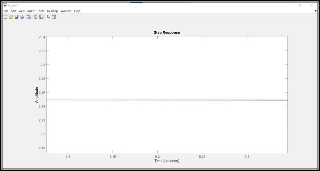
• The Peak response reaches a maximum of around 2.25 amplitude.

2)Settling time:

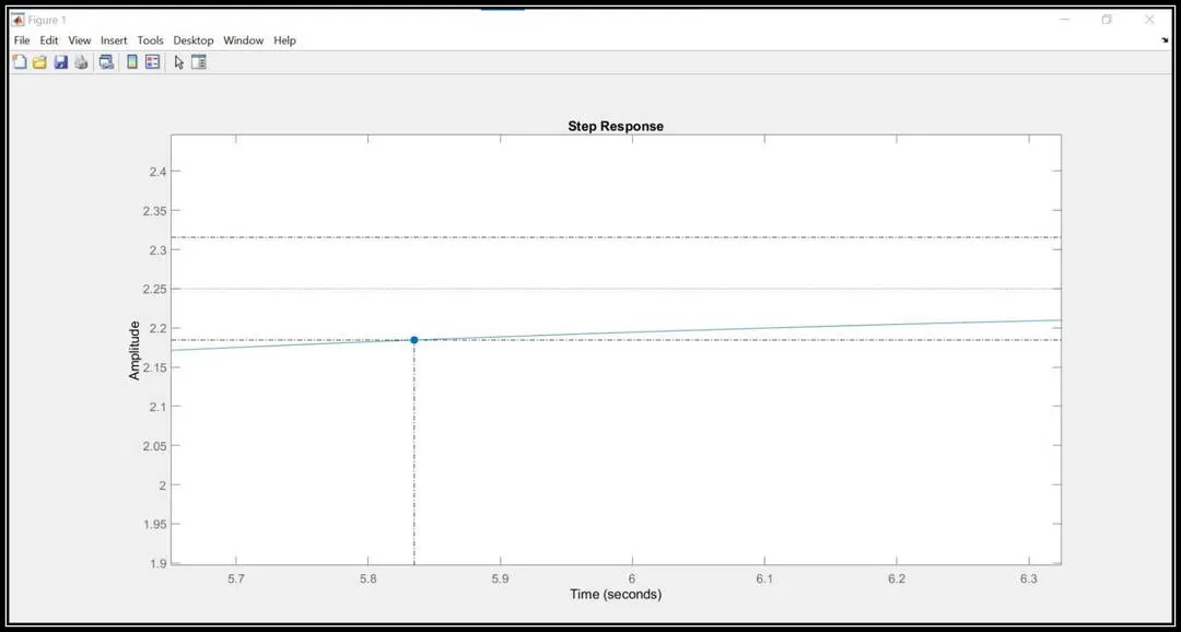
• From the above graph, it is clear that the plot reaches the settling time of 5.85 sec (approx). After the settling time, the response tries to follow the unit step. There will be no shoot out or sudden decrease after the settling time.

3)Rise Time:

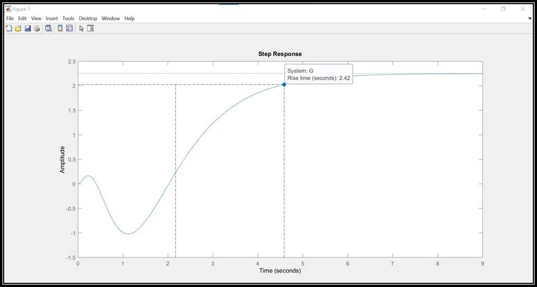
• The Rise time is the time required to reach 90% of amplitude from 10% amplitude. Here in this plot, we can observe that the rise time is 2.42 sec.

With Feedback:

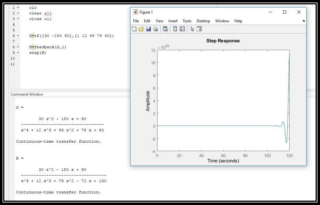
• With the feedback, the system found to be unstable and it is difficult to found the characteristic points.
• Using pid tune command in Matlab we can optimize the system to be more stable.

3)

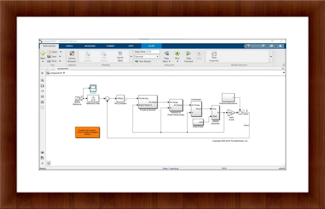
• In the above-given Engine Speed control model, all the blocks are connected in series.
• The major blocks are speed reference, PID Controller, Throtttle&manifold, Power stroke, Combustion, Drag torque, Vehicle Dynamics, and finally output.
• A Feedback loop is also present in the system which measures the output speed and gives feedback again to the PID controller.
• In the model, an additional scope is attached to the input reference speed in order to view the input speed.

1)THROTTLE&MANIFOLD SUBSYSTEM:

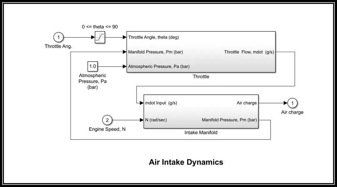
• The throttle block takes three inputs which include throttle flow(throttle angle), a manifold pressure from the intake manifold, and an atmospheric pressure of 1 bar.
• Inside the throttle block, it performs a series of calculations to find the output throttle flow, and this value is sent to the engine intake manifold along with the engine speed to obtain the air charge which is given to the power stroke block and manifold pressure which is feedback to the throttle block.
• The power stroke delay block takes the air charge and the speed (final output) as feedback to provide a certain delay to the input.

2)INDUCTION TO POWER STROKE DELAY AND COMBUSTION SUBSYSTEM:

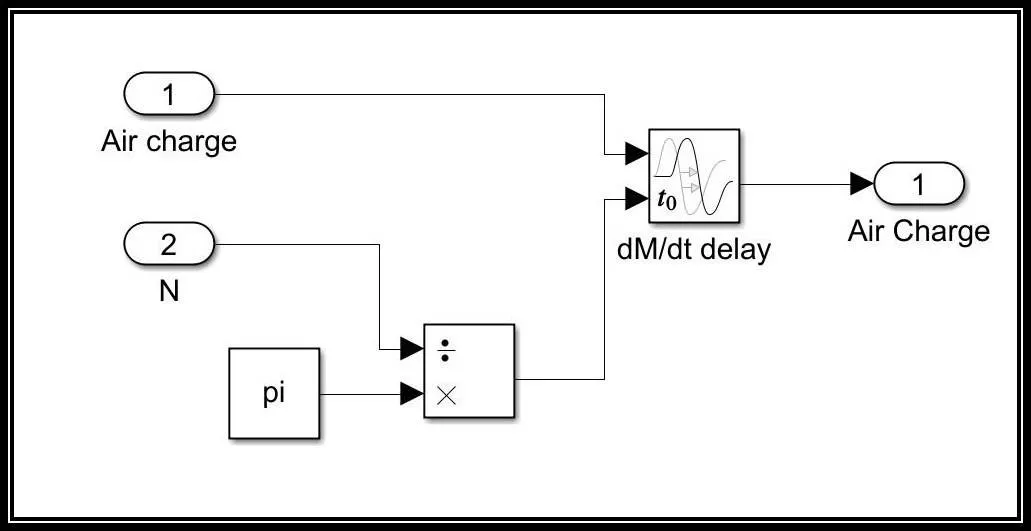
• The power stroke delay block takes the air charge and the speed (final output) as feedback to provide a certain delay to the input.

3)Combustion:

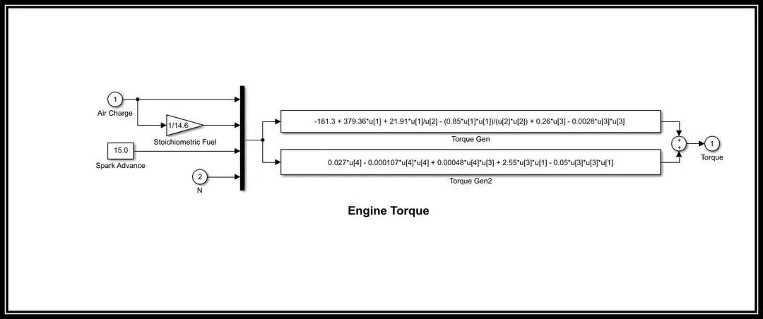
• The air charge value is converted into the fuel terms with the use of stoichiometric fuel constant along with the feedback used to find the engine torque.

4)Vehicle Dynamic Subsystem:

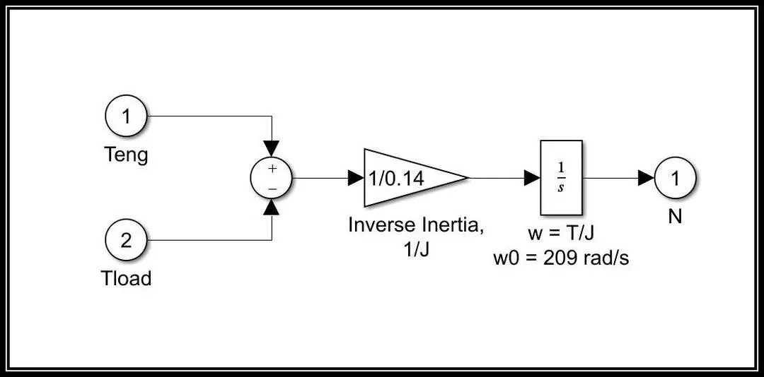
• From the engine torque, the load torque is subtracted and this value is divide by the inertia and is feed to the integrator block.
• The integration is done in order to find the value of engine speed.
• The output speed and this calculated speed is given as input to the PID controller.
• The PID controller controls the speed of the engine with the help of the reference speed given as input in the form of a step function.

PID Non-Tuned response:

• The speed control model is opened and using the default values the model is simulated.

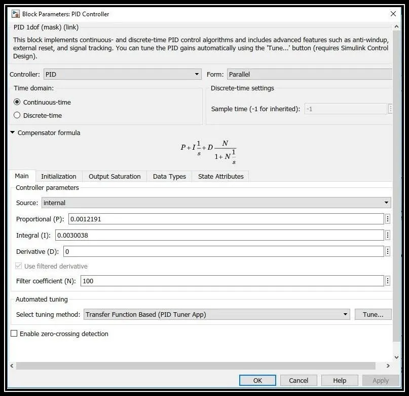
• These are the default values in the PID controller for this model.

Result:

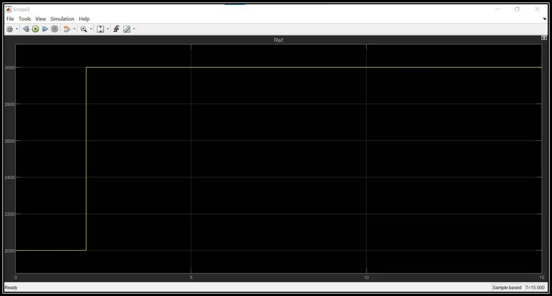
• The below image is the output of the input reference speed.

Without Tuning:

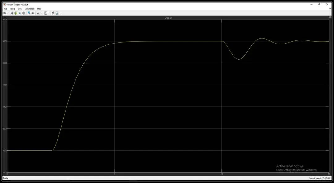
• The rise time is high which indicates that the response time to react according to the input response is high.
• From the above-mentioned figure, it shows clearly that at 2sec the response suddenly reaches 3000 but the actual output response almost takes 5 sec to reach 3000.
• For better operating behaviour and to react quickly and efficiently according to the input speed we need to tune the PID controller by changing the values of P, I, and D.

After Tuning:

• In the PID controller block using the tune option the P, I, and D values are changed.
• After updating the values the simulation is done and the below image is the output got after the changes in the values.

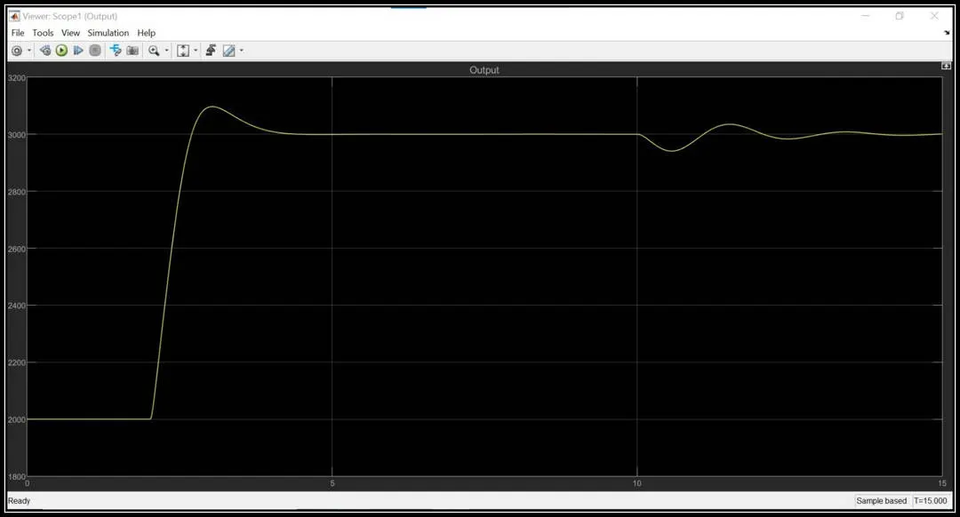
• After tuning the response time decreases rapidly and it almost tries to cope up with the input reference speed.
• In this way, the PID controller is tuned optimally to satisfy the needs.
• Even though a slight overshoot occurs, here we focus more on response time so we accept it.
• For the further best response time and minimizing overshoot fine-tune is required.

4)Importance of Bode plot:

Frequency response analysis of control systems can be carried after either analytically or graphically. The various graphical techniques available for frequency analysis are

• Bode plot
• Root locus
• Polar plot
• M and N circles
• Nichols Chart

Bode Plot:

Bode plots are usually drawn for the open-loop systems. From the open-loop plot, the performance and stability of the closed-loop system are estimated. Frequency response plots are used to determine the frequency domain, to study the stability of the systems, and adjust the gain of the system to satisfy the desired specifications. In control engineering, a bode plot is the frequency response of a system represented using two sub-plots-Magnitude plot(expressing the magnitude in decibels) and the Phase plot(expressing the phase shift in degrees.).

Determine the stability of the system using Bode plot parameters:

The stability of a control system is defined as the ability of any system to provide a bounded output when a bounded input is applied to it. More specifically we can say that stability allows the system to reach the steady-state and remain in that state for that particular input even after variation in the parameters of the system.

The stability of the system using a bode plot can be expressed in terms of gain margin and phase margin.

Gain Margin:

Greater will be the gain margin greater will be the stability of the system. It refers to the amount of gain, which can be increased or decreased without making the system unstable. It usually expressed n db.

Phase Margin:

Greater will be the phase margin greater will be the stability of the system. It refers to the phase which can be increased or decreased without making the system unstable. It usually expressed in degree.

Bode Stability Criterion:

The stability conditions are given below

• For a Stable System: Both the margins should be positive or the phase margin should be greater than the gain margin for the system to be stable.
• For Marginal Stable System: Both the gain and phase margins should be zero or the phase margin should be equal to the gain margin then the system is said to be marginally stable.
• For Unstable System: If either of the phase margin or gain margin is negative or the phase margin is less than the gain margin then the system is unstable.

Advantages of a Bode Plot:

• It is based on the asymptotic approximation, which provides a simple method to plot the logarithmic magnitude curve.
• The multiplication of various magnitude appears in the transfer function can be treated as an addition, while division can be treated as subtraction as we are using a logarithmic scale.
• With the help of this plot, we can directly comment on the stability of the system without doing any calculations.
• Bode plots provide relative stability in terms of gain margin and phase margin.
• It also covers from low frequency to high-frequency range.

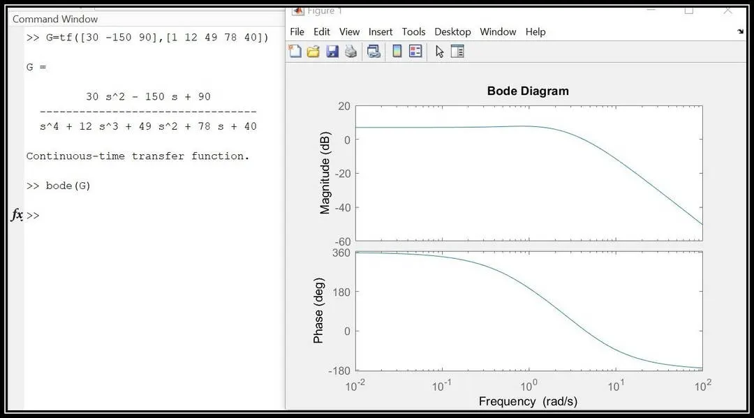
Bode plot of Transfer function:

Reference:

https://skill-lync.com/knowledgebase/how-does-a-bode-plot-determine-the-stability-of-a-system

The abovementioned article is referred to as the study of the Bode plot.