Basics of ML & AL Week 2 Challenge

week2

Q2. It is true that simple mean is sufficient enough for having an idea about the data by computing with it's formula (Sum of all observations/number of observations). But, by foregoing this computation we assume that the possibility of each event happening is equal and hence we directly compute them by summing them and taking their average. But, what if the occurance of all the events arent given? Assume we have 4 events possibly to occur namely A B and C. So we aren given with their number of occurance in difinite numbers say, A happens for 4 times, B happens for 8 times and so on. For this scenario simple mean itself is enough. But, whatif instead of their number of occurance, their probability is given? Take for example, possibility of A to occur is 0.48, possibility of B to occur is 0.31 and for C 0.21. This would get us to a point where we need to consider the weight of the event. As given in the example above, the probability of A is more than B and C. That means when we correlate this with its occurance, we can infer that the mean or the ideal possibility of the event to occur would be closest to that of A and farther from C(Holding the least probability) Imagine having more random variables and complex probability values. That is when the significance of expected mean value overcomes the simple mean value. As explained in the previous question, instead of summing the probability, we should consider the weight of each event before averaging them.

Note: The sum of the probabilities should always be 1.

Q3. Skewness is a data characteristic which measures the symmetricity of the curve. It is neither good nor bad for the analysis.

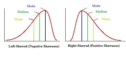
For a normal distribution, the mean, median and mode coincide. However, this is an ideal case and most of the real data have either postive or negative skewness.

A positive skewness indicates that the median and mode are greater than the mean value. On the other hand, for a negatve skewness, the mean value is higher than the median and mode.

Q4.

Z-score = (X – mean) / standard deviation.

1. P(X<711)

The z-score of this would be = (711-680)/31 = 1.

Hence, it is one standard deviation away from the mean in the positive x axis.

In the z-table, the probability value for z = +1 is 0.8413 which is 84.13%.

2. P(X>740)

The z-score of this would be = (740-680)/31 = 1.93.

Hence, it is 1.9 times the standard deviation away from the mean in the positive x axis.

In the z-table, the probability value for z = +1.93 is 0.9732.

But it is asked for probability greater than 740. Hence, we get the value until 740 and subtract from 1.

So, the final probability value = 1 - 0.9732 = 0.0268 or 2.68%.

3. P(600<x<720)< strong=""></x<720)<>

In this case, we need to find the value of probability at X<720 and X<600 and subtract both values.

When X = 720, z = 1.29 and probability value is 0.9015

When X = 600, z = -2.58 and probability value is 0.00494

Final probability value = 0.9015 – 0.00494 = 0.89656 or 89.656%.

4. P(X=720)

P(Z = 1.29) = P(1.29 < Z < 1.29) `

Since, our primary aim is to compute the area of the curve whether it is to the left or right depends on its position and if it is greater or lesser.

Hence, being a single line the area enclosed by it is Zero.

P(Z = 1.29) = P(Z < 1.29) - P(Z < 1.29)

P(Z = 1.29) = 0.9032 - 0.9032

P(Z = 1.29) = 0.

Q5. Explain the curve on the right side?

The graph given below shows the normal distribution of the data points by plotting the z-values with their corresponding probability values.

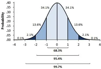
Here, the mean of this observation data is always 0 and the standard deviation is 1.

It gives us the percentage of data falling under every 1, 2 and 3 standard deviation from the mean value.

In this figure, 68.2% of data falls from z values -1 to +1, 95.4% from -2 to +2 and 99.6% from -3 to +3.

An example application of this graph would be the results of IQ test of people living in a city.

It can be noted that not everyone would have gotten the highest IQ or the lowest. Most of the range would be around the mean value which is depicted by this graph. Another example would be marks obtained in a test. It can be observed that people who score centum and people who scored a zero would be very less. More students’ marks would be around the average class mark.