Basics of ML & AL Week 2 Challenge
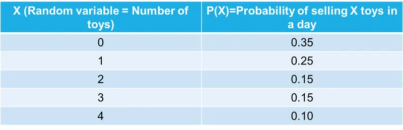
Q.1)Calculate all 4 business moments using pen and paper for the below data set?
1.First buisness moment - mean or expected value
- It is the measure of central tendency and can be calculated by formula as:
`u=sumx.P(x)`
`u=[(0times0.35)+(1times0.25)+(2times0.15)+(3times0.15)+(4times0.10)]`
`u=1.4`
2.Second buisness moment-Variance
- It is the measure of despersion.This is calculated by determining the variance of the data
- Variance,
`sigma^2=sum(X_i-u)^2.P(X)`
`sigma^2=[(0-1.4)^2times0.35+(1-1.4)^2times0.25+(2-1.4)^2times0.15+(3-1.4)^2times0.15+(4-1.4)^2times0.10]`
directly calculating using calculator
`sigma^2=1.8496` - variance
`sigma = 1.36` - standard deviation
3.Third buisness moment - skewness
- Skewness is a measure of the symmetry in distribution.it is further divided into types i.e positive skewness and negative skewness.For notmal distribution it is zero.
- skewness calculated by using formula as below.
`S_k = sum((X_i-u)/sigma)^3.P(X)`
`S_k = [((0-1.4)/1.36)^3 times0.35+((1-1.4)/1.36)^3 times0.25+((2-1.4)/1.36)^3 times0.15+((3-1.4)/1.36)^3 times0.15+((4-1.4)/1.36)^3 times0.10]`
Using calculator we get
`S_k= 0.57`
4.Fourth Buisness moment-Kurtosis
- It is a measures of combined sizes of the two tails.It measures amont of probabilty in the tails.
- It focuses on the tails of the distribution and explains whether the distribution is flat or rather with a high peak.
- The value is often compared to the kurtosis of the normal distribution
- For a normal distribution, the value of Kurtosis equals 3.
- If Kurtosis<3 then dataset have Lighter tails than normal distribution
- If Kurtosis>3 then dataset have heavier tails than normal distribution
- Kurtosis calculated by formula
`K_t = sum((X_i-u)/sigma)^4.P(X) -3`
`K_t = {[((0-1.4)/1.36)^4 times0.35]+[((1-1.4)/1.36)^4 times0.25]+[((2-1.4)/1.36)^4 times0.15]+[((3-1.4)/1.36)^4 times0.15]+[((4-1.4)/1.36)^4 times0.10]}-3`
`K_t =-0.97`
Q.2 What is the significance of expected value when simple mean (Sum of all observations/number of observations) is already in place
- Expected value and mean both are same but we use these terms in different situations.
- Situation_1: suppose A,B,C,D and their occurrences are given in this scenario simple mean itself is enough.
- But what if instead of number of occurrence their probability is given.
- For example situation_2: probability of A occur is 0.50, probability of B occur is 0.29, for C is 0.21 and so on…
- In such situation we calculate mean of probability distribution and this is known as expected value.
- Let us understand these terms with examples.
Mean
- Mean is calculated by summing all observation divided by number of observation
- Mean is typically used when we want to calculate the average value of a given sample. This represents the average value of raw data that we have already collected.
- `Mean = (sum X_i)/n`,where `X_i`= raw data values , n = sample size
- Suppose we record the number of goals that a soccer team scores in 15 different games
- Goal scored:1,1,0,2,2,1,0,3,1,1,1,2,4,3,1
- By using above formula : mean number of goals scored /game by team
- `Mean = (1+1+0+2+2+1+0+3+1+1+1+2+4+3+1)/15=1.533`goals
- This represents the mean number of goals scored per game by the team
Expected value
- Expected value is used when we want to calculate the mean of a probability distribution. This represents the average value we expect to occur before collecting any data.
- `Expected value = sum X* P(x)`,where X=Data value, P(X) = probability of value
- For example, probability distribution tells us the probability that certain soccer team scores certain number of goal in given game.
Goals(x) Probability P(x) 0 0.18 1 0.34 2 0.35 3 0.11 4 0.02 - By using above formula :Expected value (mean)for this probability distribution
- `Expected Value= 0*0.18+1*0.34+2*0.35+3*0.11+4*0.02=1.45`goals
- This value represents the number of goals that the team will score in any game.
Q.3.Having skewness in the curve considered to be bad in the analysis?
- Skewness is the measure of how much the probability distribution of random variables from the normal distribution.
- A data is called as skewed when curve appears distorted or skewed either to the left or to the right, in the statistical distribution.
- In a normal distribution, graph appears symmetrical on both sides of the median. Also in normal distribution mean, median and mode are approximately closer. And these three are all measure of center of data.
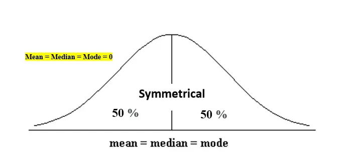
- The skewness of the data can be determined by how these quantities are related to each other.
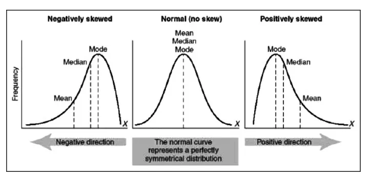
- There are two types of skewness i.e positive and negative skewness
- The probability distribution with its tail on right side is a positively skewed distribution and the one with its tail on the left side is negatively skewed distribution.
- When mean=median=mode - skewness is zero then graph shows the normal distribution.”
- When mode >median>mean -negatively skewed
- When mean > median > mode –positively skewed
- I don't think wheather having skewness is good or bad,we can't determine wheather it is good or bad.
- rather than worrying about it is good or bad .we must focus on knowing about skewness .It help us to understand the characterstics of data set.
- In Real life distributions are usually skewed. If there are too much skewness in the data, then many statistical model don’t work
- Because in skewed data, the tail region may act as an outlier for the statistical model and we know that outliers adversely affect the model’s performance especially regression based models.
- There is necessity to transform the skewed data to close enough to Gaussian distribution or normal distribution.
- Linear models works on the assumption that the distribution of the independent variable and target variable are similar so it becomes important to know about the skewed data. It helps us in creating better linear model.
Q.4 Evaluate the probabilities for continuous normal distribution with given mean = 680 and standard deviation = 31
a)P(X<711)
b)P(X>740)
c)P(600<x<720)< p=""></x<720)<>
d)P(X=720)
solution :
- To evaluate the probability of contineous normal distribution,
- first we calculate z score value from given mean and standard deviation by using formula
- Z -score = (X-mean) / standard deviation
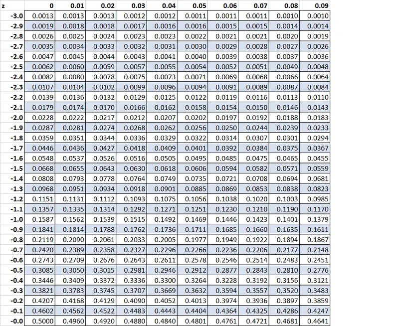
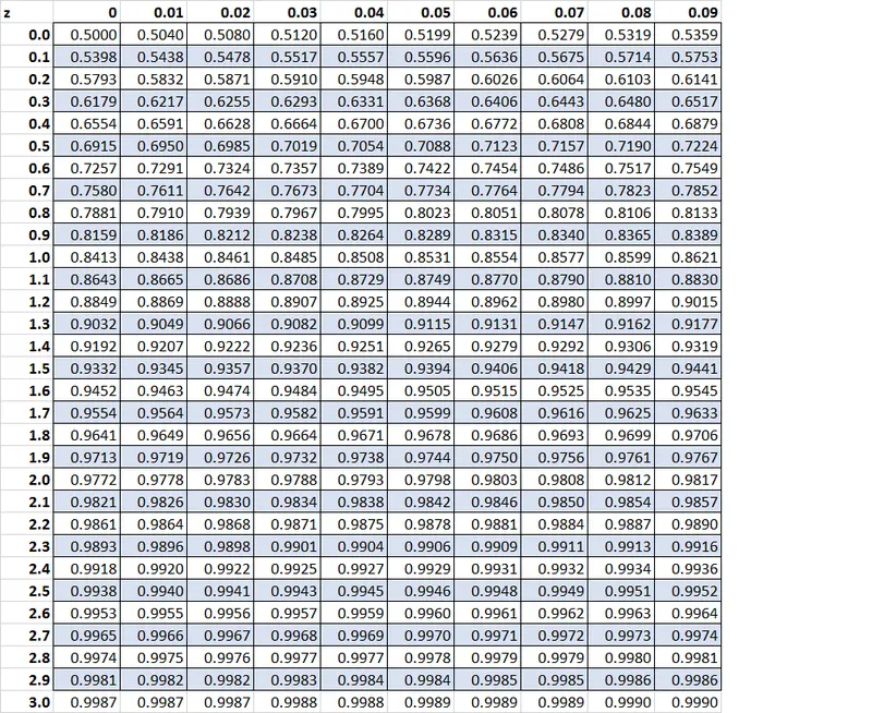
- then the z values are looked into the z-table to identify the probability less than or equal to that value.
1.P(X<711)
step 1 : find z-score
`z=(711-680)/31=1`
- It is one standard deviation away from the mean in the positive x axis ,
step 2 : Use the z-table to find the percentage that corresponds to the z-score.
- in the z table ,the probabilty value for z=+1 is 0.8413 which is 84.13%
2.P(>740)
step 1 : find z-score
`z-score =(740-680)/31=1.93`
- It is 1.9 times the standard deviation away from the mean in the positive x axis
step 2 : Use the z-table to find the percentage that corresponds to the z-score.
- In the z - table probability value for z=+1.93 is 0.9732
3.P(600<X<720)
step 1 & step 2 : find z-score and probabilty
- In this case, we need to find the value of probability at X<720 and X <600 and substract both values
- When X= 720 ,`z-score =(720-680)/31=1.29` and probability value for z-score =1.29 is 0.9015
- when X = 600,`z-score =(600-680)/31=-2.58`,and probability value for z-score =-2.58 is 0.0049
step 3: substract both values
P(600<X<720) = P(X<720)-P(X<600)
= 0.9015-0.0049
=0.8966 or 89.66%
4.P(X=720)
- It is not possible to calculate area for x=720 exact value ,any ways it leads to zero as distribution is contineous.
- Since the area under any curve corresponding to a single point is (for practical purposes) zero, the probability of obtaining exactly a specific value is zero
- our primary aim is to calculate area under wheather it is left or right (or less or greater).but in this case being single line the area enclosed by it is zero
- Let us see by actaual calculation
step 1:find z-score
`z-score = (720-680)/31=1.29`
step 2 : Use the z-table to find the percentage that corresponds to the z-score.
z-score =1.29
P(z=1.29)=P(z<1.29)-P(z<1.29)
=0.9032-0.9032=0
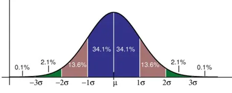
5)Explain the curve on the right side
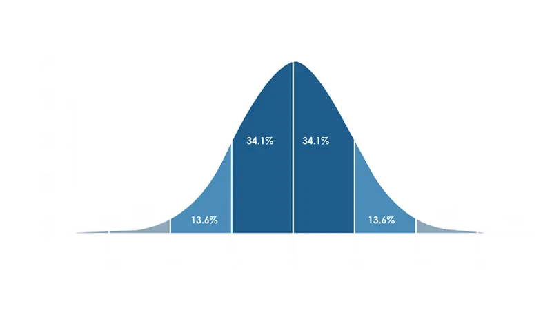
- The given curve is Normal distribution also called the bell curve or Gaussian distribution. Normal distribution is bell shaped and symmetric about a vertical line through its center. Mean, median and mode are all equal and located at the center of the distribution.
- The curve is symmetric at the center (i.e., around the mean, μ)
- Exactly half of the values are to the left of center and exactly half the values are to the right.
- The total area under the curve is 1.
- In a normal distribution graph, the mean defines the location of the peak, and most of the data points are clustered around the mean.
- The standard deviation determines the width of the curve, and it tightens or expands the width of the distribution along the x-axis.
- smaller standard deviation indicates the data clustered tightly around the mean and normal distribution will be taller and vice versa
- we can see in above bell curve percentage shows the area covered under the curve and divisions along the x axis shows standard deviation and central line is mean.
- If you see on either side of mean(i.e `1 sigma` ) 34.1 + 34.1 = 68.2 % of data falls within one standard deviation.
- `2sigma` taken on either side of mean 34.1 + 34.1+13.6+13.6 = 95.4% of data falls betwen `-2sigma` to `+2sigma`
- from `-3sigma`to `+3sigma` data falls within this range will equals to 34.1 + 34.1+13.6+13.6+2.1+2.1=99.7%
- For clarity, see the below curve.