Basics of ML & AL Week 2 Challenge

Assignment -2

1. Calculate all the four business moments:

x	p(x)	(A) = x*p(x)	Variance	Skewness	Kurtosis
0	0.35	0	0.686	-0.38479	0.397141
1	0.25	0.25	0.04	-0.00641	0.00189
2	0.15	0.3	0.054	0.012981	0.005742
3	0.15	0.45	0.384	0.246164	0.290359
4	0.1	0.4	0.676	0.704196	1.349764
	E(x) =	1.4	1.84	0.572139	-0.9551

The answers are highlighted in bold in the last row of the above table.

2. What is the significance of expected value when a simple mean (Sum of all observations/ number of observations) is already in place?

Mean is defined as the sum of individual observation divided by the number of observations in the collection.

Mean= 1/n ∑Xi

Expected value (EV) is the probability of an event multiplied by the amount of times the event happens.

EV=∑P(Xi​)×Xi​​

For example:

In the case of a fair dice, it is easy to see that the mean and the EV are the same.

Mean of possible outcomes - (1+2+3+4+5+6)/6 - 3.5

and EV would be:

Outcome (X)	Probability (P(X))	X*P(X)
1	1/6	1/6
2	1/6	1/3
3	1/6	1/2
4	1/6	2/3
5	1/6	5/6
6	1/6	1
Expected value =		3.50

EV= ∑P(Xi​)×Xi​​ = 3.50

But what if the dice were not "fair." An easy way to make an unfair die would be to drill a hole in the corner at the intersection of the 4, 5, and 6 faces. Further let's now say that the probability of rolling a 4, 5, or 6 on our new and improved crooked die is now 0.2 and the probability of rolling a 1, 2, or 3 is now 0.133. It is the same die with 6 faces, one number on each face, and the mean for this dice is still 3.5. However, after rolling this die many times, our EV is now 3.8 because the probabilities for the events are no longer the same for all events.

Outcome (X)	Probability (P(X))	X*P(X)
1	1/8	0.13
2	1/8	0.27
3	1/8	0.40
4	1/5	0.80
5	1/5	1.00
6	1/5	1.20
Expected value =		3.80

EV = 3.80

A probability distribution defines the relative frequency of outcomes of a random variable - the expected value can be thought of as a weighted average of those outcomes (weighted by the relative frequency). Similarly, the expected value can be thought of as the arithmetic mean of a set of numbers generated in exact proportion to their probability of occurring (in the case of a continuous random variable this isn't exactly true since specific values have probability 0).

3. Having skewness in the curve is considered to be bad in the analysis?

Skewness is defined as the degree of distortion from the symmetrical bell curve or the normal distribution. It measures the lack of symmetry in data distribution.
It differentiates extreme values in one versus the other tail. Asymmetrical distribution will have a skewness of 0.

There are two types of Skewness: Positive and Negative

Positive Skewness means when the tail on the right side of the distribution is longer or fatter. The mean and median will be greater than the mode.

Negative Skewness is when the tail of the left side of the distribution is longer or fatter than the tail on the right side. The mean and median will be less than the mode.

The rule of thumb seems to be:

• If the skewness is between -0.5 and 0.5, the data are fairly symmetrical.
• If the skewness is between -1 and -0.5(negatively skewed) or between 0.5 and 1(positively skewed), the data are moderately skewed.
• If the skewness is less than -1(negatively skewed) or greater than 1(positively skewed), the data are highly skewed.

Having skewness is not considered to be bad, it depends on the type of distribution that we analyze. Skewness is an attribute to describe the distribution.

4.

1. i) P(X<711) =

711 = 680 (Mean) + 31 (Standard Deviation)

So probability of X<711 = Sum of probability less than mean (0.50) + Probability up to one standard deviation(σ) i.e 31

= 0.50 + 0.341

= 0.841

1. ii) P(X>740) =

Calculating Z score = (x-µ)/σ

Z = (740 – 680)/31

= 1.9354

From Z table the probability for 1.93 = .9732

.9732 gives the probability up to 740. We need P(X>740) So, we subtract the probability up to 740 from 1 (Since the total probability is 1)

Therefore P(X>740) = 1-0.9732 = 0.0268

iii) P(600<X<720)

We calculate Z score for X = 600 & X = 720 we subtract the area (probability) of X = 600 from X= 720 to get the probability between 600 and 720.

For P(X = 720), Z = (720 – 680)/31 = 1.29

When Z = 1.29 probability from Z tables = 0.9015

For P(X = 600), Z = (600 – 680)/31 = -2.58

When Z = -2.58 probability from Z tables = 0.0049

Therefore = P(600<X<720) = P(X<700) – P(X<600) = 0.9015 - 0.0049 = 0.8966 (ANS).

1. iv) P (X = 720)

The probability of X = 720 is equal to the area under X =720 which is infinitesimally small.

Therefore, P(X = 720) = 0

5. Explain the normal distribution curve.

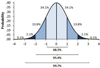
The above figure is the normal distribution curve which shows the probability distribution. The total area under the curve represents the total probability i.e equal to 1. Zero on x- axis represents the mean value and 1 represents one standard deviation from the mean and -1 represents negative standard deviation that is one standard deviation away from the mean.

When we have normally distributed data, the standard deviation becomes particularly valuable. we can use it to determine the proportion of the values that fall within a specified number of standard deviations from the mean. For example, in a normal distribution, 68% of the observations fall within +/- 1 standard deviation from the mean. This property is part of the Empirical Rule, which describes the percentage of the data that fall within specific numbers of standard deviations from the mean for bell-shaped curves.

Mean +/- standard deviations	Percentage of data contained
1	68%
2	95%
3	99.7%

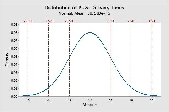
Let’s look at a pizza delivery example. Assume that a pizza restaurant has a mean delivery time of 30 minutes and a standard deviation of 5 minutes. Using the Empirical Rule, we can determine that 68% of the delivery times are between 25-35 minutes (30 +/- 5), 95% are between 20-40 minutes (30 +/- 2*5), and 99.7% are between 15-45 minutes (30 +/-3*5). The chart below illustrates this property graphically

6. Explain kurtosis?

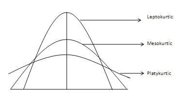
Kurtosis is all about the tails of the distribution — not the peakedness or flatness. It is used to describe the extreme values in one versus the other tail. It is actually the measure of outliers present in the distribution.

High kurtosis in a data set is an indicator that data has heavy tails or outliers. If there is a high kurtosis, then, we need to investigate why do we have so many outliers. It indicates a lot of things, maybe wrong data entry or other things.

Low kurtosis in a data set is an indicator that data has light tails or lack of outliers. If we get low kurtosis (too good to be true), then also we need to investigate and trim the dataset of unwanted results.

Types of kurtosis:

Meso-kurtic: This distribution has kurtosis statistics like that of the normal distribution. It means that the extreme values of the distribution are similar to that of a normal distribution characteristic. This definition is used so that the standard normal distribution has a kurtosis of three.
Lepto-kurtic (Kurtosis > 3): Distribution is longer, tails are fatter. Peak is higher and sharper than Mesokurtic, which means that data are heavy-tailed or profusion of outliers.
Outliers stretch the horizontal axis of the histogram graph, which makes the bulk of the data appear in a narrow (“skinny”) vertical range, thereby giving the “skinniness” of a leptokurtic distribution.
Platykurtic: (Kurtosis < 3): Distribution is shorter, tails are thinner than the normal distribution. The peak is lower and broader than Meso-kurtic, which means that data are light-tailed or lack of outliers.
The reason for this is because the extreme values are less than that of the normal distribution.

Its significance can be explained using an example. In finance, if the investment returns are leptokurtic then the investments are prone to extreme values on either side. Whereas a platykurtic distribution is preferred in investments because the probability of extremities is less.