Basics of ML & AL Week 2 Challenge

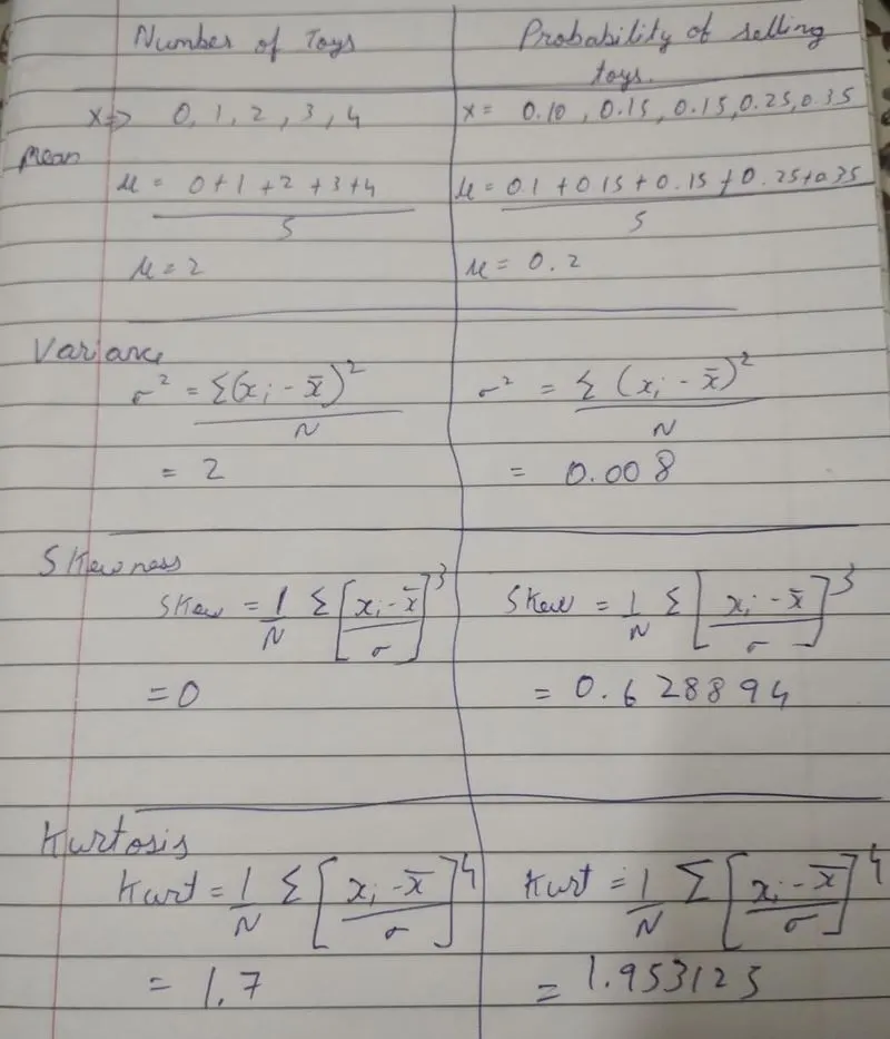
1)Calculate all 4 business moments using pen and paper for the below data set?

 -- 

2)What is the significance of expected value when simple mean (Sum of all observations/number of observations) is already in place

-- Expected value is a concept in probability theory that represents the average outcome of a random event over a large number of trials. It is calculated by multiplying the probability of each possible outcome by its associated value, and then summing these values. The expected value is denoted as E(X), where X is the random variable.

While the simple mean is a measure of central tendency that represents the arithmetic average of a set of observations, the expected value takes into account the probabilities of different outcomes and their associated values.

For example, consider a coin flip where there is a 50% chance of getting heads and a 50% chance of getting tails. The simple mean of this random event would be 0.5, which is the arithmetic average of the possible outcomes. However, the expected value of the coin flip would be (0.5 x 1) + (0.5 x 0) = 0.5, which takes into account the probabilities and values of the outcomes.

The expected value is useful in situations where there are multiple possible outcomes with different probabilities and associated values. It can help in making decisions by providing a more accurate representation of the potential outcomes and their expected values. In summary, while the simple mean is a useful measure of central tendency, the expected value provides a more nuanced understanding of the probability distribution of a random event.

3)Having skewness in the curve considered to be bad in the analysis?

-- Having skewness in a curve is not necessarily "bad" in analysis. Skewness is a measure of the asymmetry of a probability distribution, and it can be either positive (right-skewed) or negative (left-skewed). In many cases, skewed distributions are simply a reflection of the underlying data and may be perfectly valid and useful for analysis.

However, in some situations, skewness may be undesirable. For example, if you are working with financial data and the distribution of returns is highly right-skewed, this may indicate a high risk of large losses, which could be problematic for investors. Similarly, if you are working with data on income or wealth, a highly right-skewed distribution could indicate income inequality, which may be a concern for policymakers.

In some statistical analyses, assumptions may be made about the underlying distribution of the data. For example, some statistical tests assume that the data are normally distributed. In such cases, a highly skewed distribution may violate these assumptions and make the results of the analysis less reliable.

Overall, whether or not skewness is "bad" for analysis depends on the context and the specific research question being addressed. It is important to carefully consider the properties of the data and choose appropriate statistical methods that account for any skewness that may be present.

4)Evaluate the probabilities for continuous normal distribution with given mean = 680 and standard deviation = 31

-- To evaluate the probabilities for a continuous normal distribution with a mean of 680 and a standard deviation of 31, we need to use the standard normal distribution table or a calculator with a normal distribution function.

a) P(X<711) can be found by calculating the area under the normal distribution curve to the left of x = 711.

Z-score for x = 711 is calculated as follows:

Z = (711 - 680) / 31 = 1

From the standard normal distribution table or a calculator, we can find that the probability of Z being less than 1 is approximately 0.8413. Therefore, the probability of X being less than 711 is approximately:

P(X<711) = P(Z<1) = 0.8413

b) P(X>740) can be found by calculating the area under the normal distribution curve to the right of x = 740.

Z-score for x = 740 is calculated as follows:

Z = (740 - 680) / 31 = 1.9355

From the standard normal distribution table or a calculator, we can find that the probability of Z being greater than 1.9355 is approximately 0.0269. Therefore, the probability of X being greater than 740 is approximately:

P(X>740) = P(Z>1.9355) = 0.0269

c) P(600

First, we need to calculate the Z-scores for both x = 600 and x = 720:

Z1 = (600 - 680) / 31 = -2.5806

Z2 = (720 - 680) / 31 = 1.2903

From the standard normal distribution table or a calculator, we can find that the probability of Z being less than -2.5806 is approximately 0.0050, and the probability of Z being less than 1.2903 is approximately 0.9015. Therefore, the probability of X being between 600 and 720 is approximately:

P(600

d) P(X=720) is equal to zero since the probability of obtaining an exact value in a continuous distribution is zero.

5)Explain the curve  on the right side

-- The curve on the right side of a normal distribution is the portion of the distribution that represents values greater than the mean. In a normal distribution, the curve is symmetrical, meaning that the same percentage of values fall on either side of the mean. The curve on the right side of the mean represents the positive or right skew of the distribution.

A normal distribution curve is characterized by its mean and standard deviation. The mean represents the central tendency of the distribution, and the standard deviation represents how spread out the values are from the mean. The area under the curve to the right of the mean represents the proportion of values that are greater than the mean.

If the curve on the right side of the mean is steeper or taller than the left side, then the distribution is said to be positively skewed. This indicates that there are more values on the right side of the mean than on the left side. For example, if the mean is 50 and the standard deviation is 10, and the curve on the right side of the mean is taller than the left side, this indicates that there are more values above 50 than below 50.

Overall, understanding the curve on the right side of a normal distribution can provide insight into the shape and characteristics of the data being analyzed.

To explain the curve 2 images are attached below.