Side Pole Crash Simulation Challenge

SIDE POLE CRASH SIMULATION OF DODGE NEON CAR

Project 2 – Crashworthiness Analysis Using Hypermesh, Radioss, and HyperCrash(SIDE POLE CRASH ANALYSIS)

Objective

Perform a side pole crash for a neon car modal and evaluate the standard and characteristics of the simulation

• To perform the crash analysis on the side section of the car and to check where the stresses are acting on it.
• To check the unit systems and change if necessary
• Create an interface of Type 7 with the friction value of 0.2 and other parameters.
• Make sure there aren’t any penetrations
• Correct rigid bodies for any issues
• Create a rigid wall with friction 0.1.
• Compare the model weight with the full-scale 300k nodes model and use added masses to reach the target weight of 700kg while getting CG about the required range.
• Give an initial velocity of 35 mph.
• Use a model checker to ensure good quality.
• Give the Time-step: 0.5 microseconds.
• Give Run time as 80 ms.

Output Requests:

• Sectional force in the cross member.
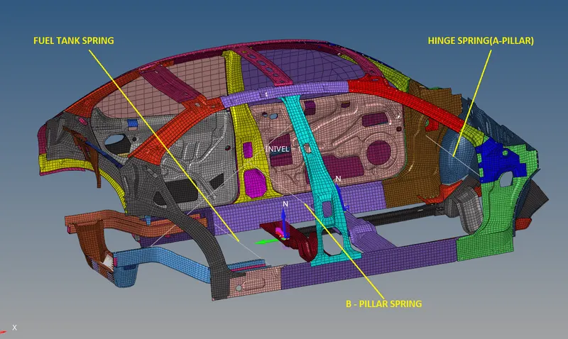
• The intrusion at B Pillar,hinge pillar & Fuel tank region
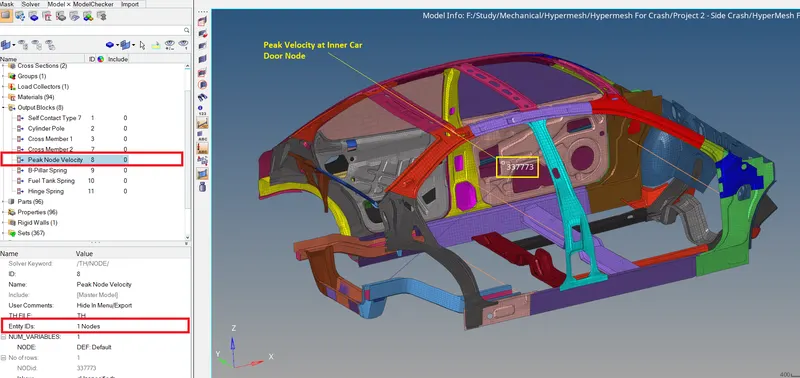
• Peak velocity of node 110643

  SIDE POLE CRASH TEST:

  

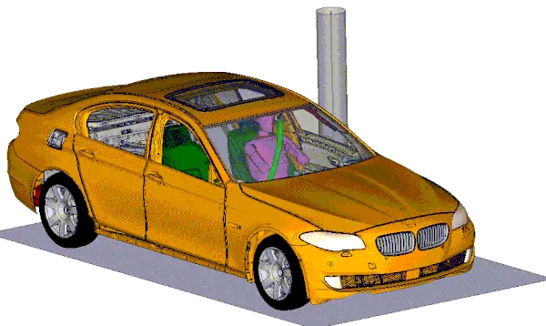
  The main reason to conduct this type of crash is to study the occupant's head Impact Criteria(HIC) and the intrusions in the underbody structures.

  There are two types of side pole tests are conducted, they are;

  Side pole crash test at 90degree,

  Side pole crash test at 75degree.

  The 90 and 75 degree both denotes the impact line of the pole towards the B pillar of the vehicle(side view).

  

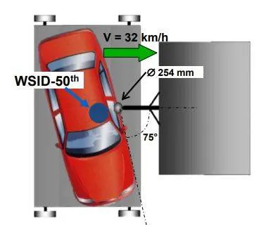
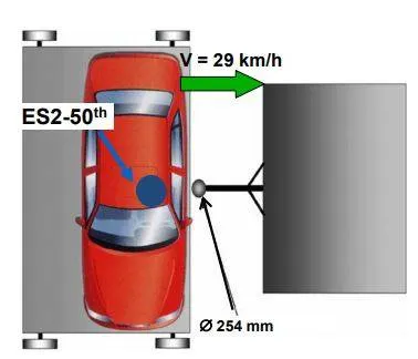
  Both of the types have different input crash criteria. At 90degree crash the car impacts the pole at the speed of 32kmph and for the 75degree crash, the car impacts the pole at the speed of 29kmph. The diameter of the side pole is 254mm and it is constant for both the types of impact.

  

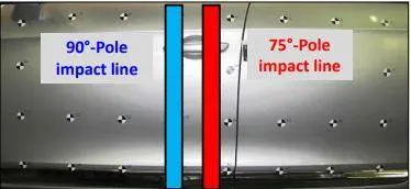
  The dummies used on both tests are different. The 75degree pole test is also known as the oblique side pole crash test. For oblique pole crash, the vehicle is offset 15degree in zaxis at counterclockwise direction of the global axis.

  BODY in WHITE(BIW):

  Body in white (BIW) is the stage in automobile manufacturing in which a car body's frame has been joined together, that is before painting and before the motor, chassis sub-assemblies, or trim(glass, door locks/handles, seats, upholstery, electronics, etc.) have been integrated into the structure. Assembly involves different techniques such as welding (spot, MIG/MAG), riveting, clinching, bonding, and laser brazing.

  

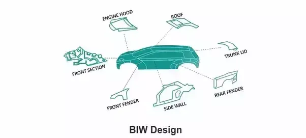
  In-car design, the BIW phase is where the final contours of the car body are worked out. Extensive computer simulations of crashworthiness, manufacturability and automotive aerodynamics are required before a clay model from the design studio can be converted into a body in white ready for production.

  de of the door.

  (F) Procedure For Side Door Of Dodge Neon Car Crash Simulation

  (1) Import Model in HyperMesh

  

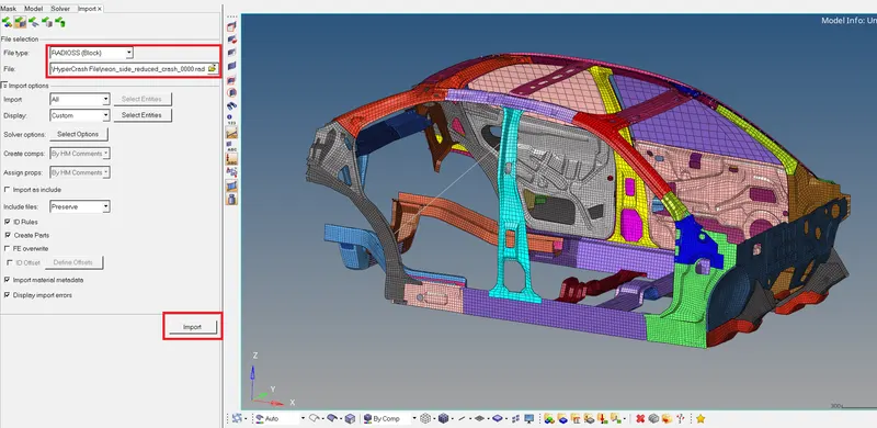
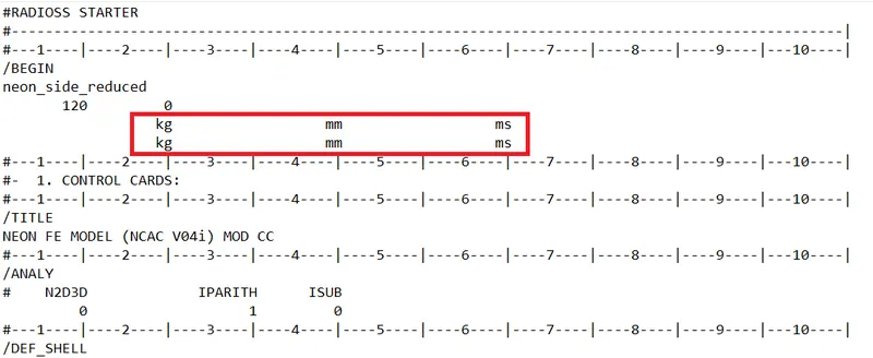
  (2) Check for Unit System

  The information provided for the crash simulation of Neon Car consists of two files are given as follows

  • neon_side_reduced_0000.rad - The file contains information about mesh nodes or element information, components of the car, material laws, contact details, boundary conditions, etc. The file is made up of ASCII type that contains the essential model information. This file is also called the starter file which always ends with 0000. rad.
  • neon_side_reduced_0001.rad– The file contains information about runtime, time step, animation frequency, no. of animation file, number and size of time history file etc. The file made up of ASCII type that describes running instruction for the solver. This file is also called the engine file which always ends with 0001. rad.

  

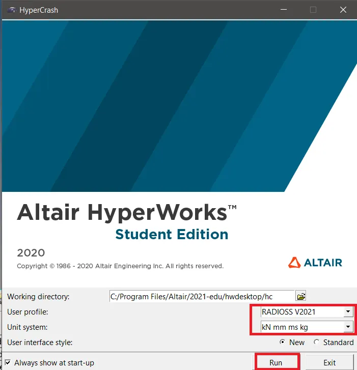
  • Important operation will be performed in HyperCrash, it will be opened by following (Application >> HyperCrash).

  

  • The starting frame of HyperCrash will be displayed with units (kN mm ms kg) taken in reference as per the units (kg mm ms) in the starter file neon_side_reduced_0000.rad and finally select the Run option to open the HyperCrash.

  

  (3) Import File in HyperCrash

  • Select starter file neon_side_reduced_0000.rad and transfer it in the HyperCrash Window Frame to open the car model.

  

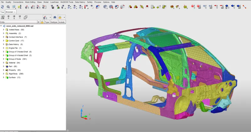
  (4) Penetration and Intersection

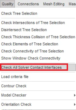
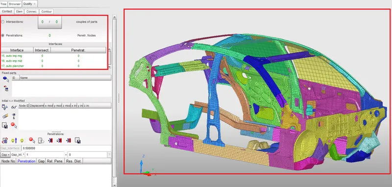
  • Penetration and Intersection operation will be performed by following (Quality >> Check All Solver Contact Interfaces). Contour window will open in which (include picked parts) option selected by following inside the fixed parts windows and finally click on the penetration option.

  

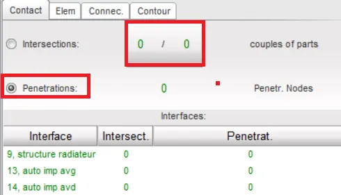
  • After performing operation, it indicates that zero evidence of intersection and penetration is present inside the model.

  

  (5) Compare model weight with fully fledged 300k model and use added masses to reach the target of 700kg weight while reaching Centre of Gravity to the required location

  • The centre of gravity for vehicle is a theoretical point at which all masses of each of its different individual components lies at one point.
  • Sunroof at the top of the vehicle will raise centre of gravity of the vehicle while center of gravity will lower by placing battery pack at the bottom of the vehicle.
  • Lower the centre of gravity better will be the handling point of vehicle during cornering and braking and also it reduces roll on.

  Added Masses

  • Addition of mass is essential in order to stabilize the centre of gravity of the car. The present model for crash simulation does not have many important components because of node limitation.
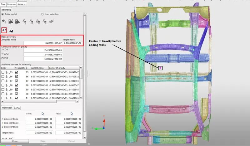
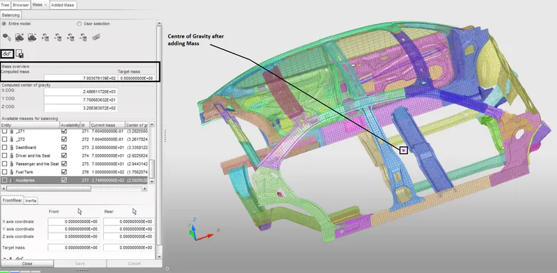
  • The checking of centre of gravity of car will be done by following (Mass >> Balancing) process. In mass window frame, click on the (Show COG point) to check where the centre of gravity available at the moment in the model.
  • In Mass overview, computed mass is 166 kg but it is required to add mass to compensate components which are not available inside the car model to reach to target of 700kg weight through added mass options.

  

  

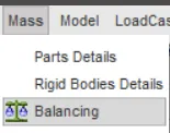
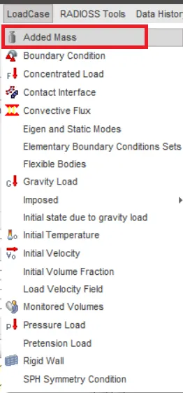
  • Added mass will be opened by following (Load Case >> Added Mass) process. In Added Mass, new mass will be created with Type 1 (Mass is disturbed to each node of node group).

  

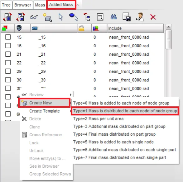
  • After Type 1, assign added mass with required kg mass and then (Right click>> select in graphics >> Add/Remove node by picking selection) as per the different components which are not available inside the car model. The mass will be added at five different locations of the car model in order to transfer center of gravity at the desired location to stabilize it.

  Weights Distribution on Car to balance COG

  Mass in kg	Description	Location
  70	Driver and his Seat	IMAGE(1)
  70	Passenger and his Seat	IMAGE(2)
  100	Fuel Tank	IMAGE(3)
  20	DashBoard	IMAGE(4)
  274	Auxiliaries	IMAGE(5)

  

  

  

  

  

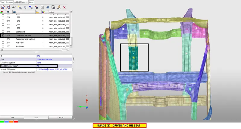
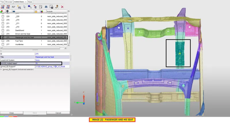
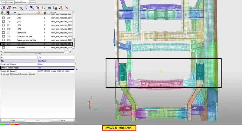
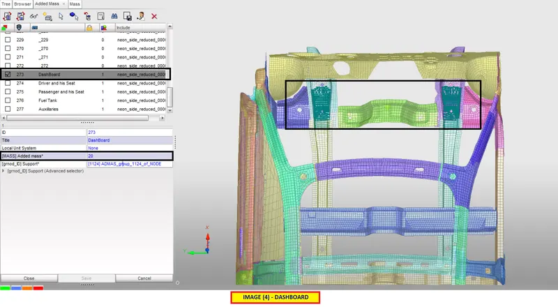
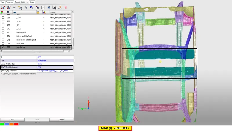
  • Below Images shows that 700kg weight target and transferring centre of gravity at the desired location has been achieved by adding mass at the different location of the car model in order to compensate absent components.

  

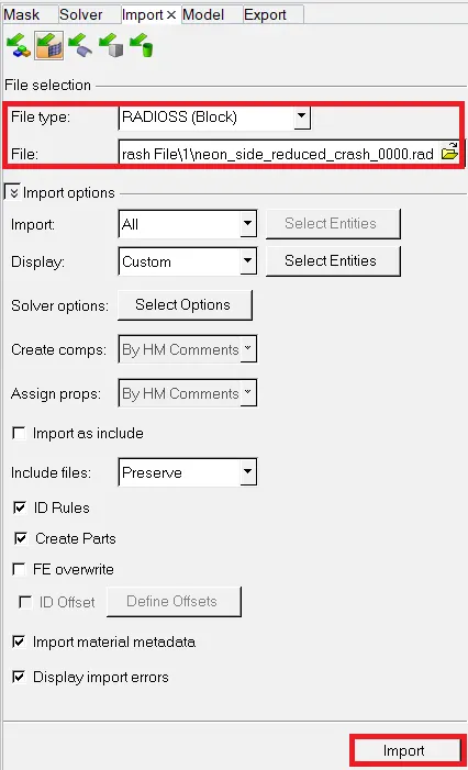
  (6) Export HyperCrash File in HyperMesh

  • After making necessary changes in the HyperCrash, file will be saved as neon_front_car_crash_0000.rad by following (File >> Export >> Radioss).
  • Import HyperCrash file in HyperMesh by following the (File >> Import) process.

  

  (7) Contact Interface

  • In this case, the Type 7 Contact Interface is defined. Interface TYPE7 is a multi-usage impact interface, modelling contact between a master surface and a group of slave nodes. It is also possible to consider heat transfer and heat friction.

  All limitations that were encountered with interfaces TYPE3, TYPE4 and TYPES are solved with this interface:

  • A node can at the same time be a slave and a master node.
  • Each slave node can impact each master segment; except if it is connected to this segment.
  • A node can impact more than one segment.
  • A node can impact on the two sides, on the edges and on the corners of each segment.
  • It is a fast search algorithm without limitations.

  The main limitations of this interface are:

  • Time step is reduced in case of high impact speed or contacts with a small gap.
  • It does not work properly if used with a rigid body at high impact speed or a rigid body with a small gap.

  It does not solve edge to edge contact (to solve this, /INTER/TYPE11 should be used along with TYPE7).

  Interface Type7: Nodes to Surface Contact

  • It is the node to surface contact and it is a universal type of contact.
  • A gap is defined around the master segment and slave nodes and this gap can be variable or constant.
  • The slave is kept outside of the master gap by resistive force application.

  Advantages:

  • Type 7 interface is non-oriented and slave nodes can belong to the master surface unlike type 3 and 5.
  • The search of the master or slave segment is carried out using a direct search algorithm.
  • Energy jumps because of Edge impact are removed by cylindrical gaps around edges.
  • Has variable stiffness and the stiffness is not constant throughout. Due to this, instability because of node penetration through thickness is removed.

  Recommended Type 7 Options

  

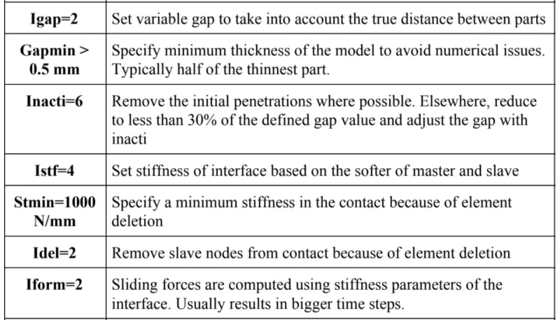
  • As we are considering self-contact for the car model, slave and master segments for this type 7 contact for the entire car model. The selection of all components under the slave and master segments respectively are given as below

  

  

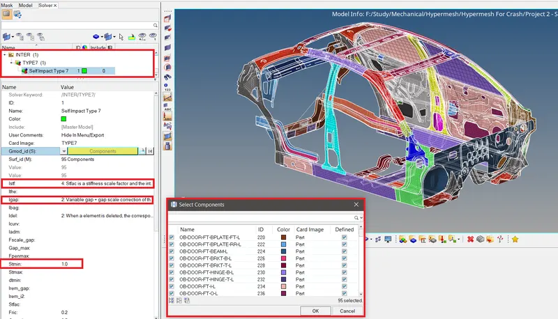
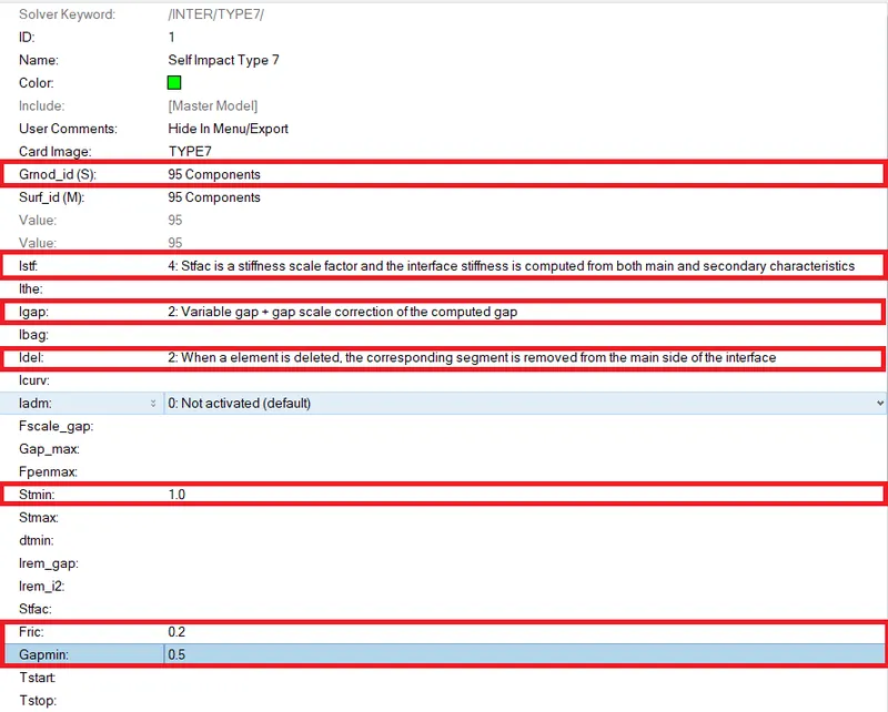
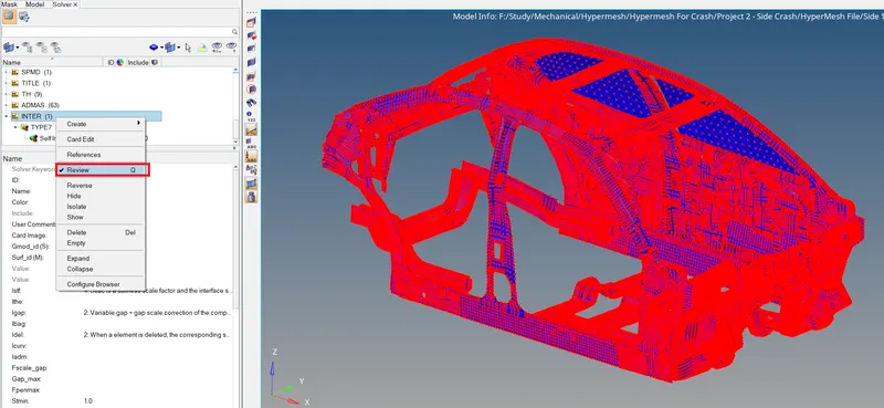
  • Reviewing the selection of nodes of all components of vehicle model by (Inter >> Right Click >> Review(Q)) process shown below

  

  (8) Rigid Wall

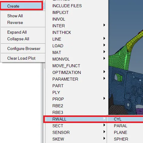
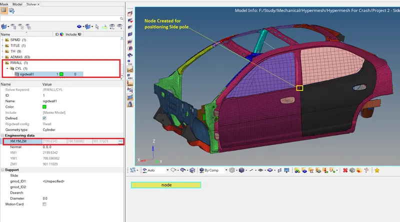
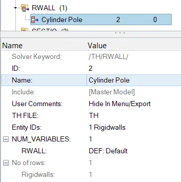
  • Now Rwall window frame will be created by following (Solver >> Right Click >> RWALL>> CYL) process.

  

  • The node will select on the corner of the front side door of the car model.
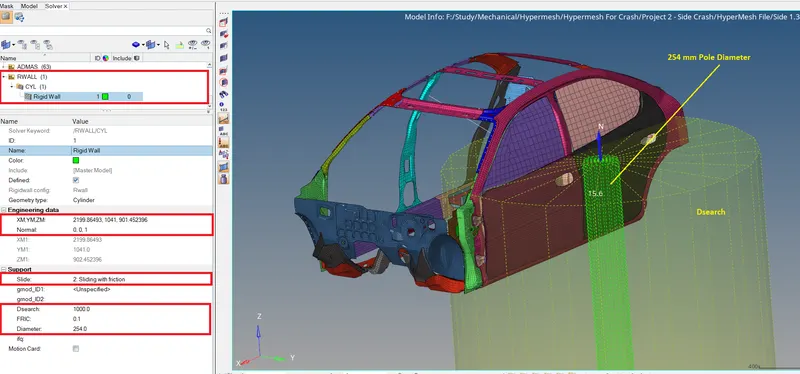
  • The side pole is facing opposite to the side door of car model with normal to the z-axis representation. When slave node comes in contact, frictional parameter will be provided for the car model.

  

  • In support frame, slide of sliding with friction and coulomb friction of 0.1 will be provided. D-search basically distance for secondary search represents all the node within the range of d-search distance considered as slave node for the contact between the rigid wall and car model with value of 1000 m. The diameter of side pole will provide with value of 254 mm.

  

  (9) Initial Velocity

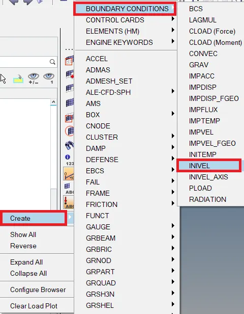
  • Initial velocity will be opened by following (Solver >> Right Click >> Create >> BOUNDARY CONDITIONS >> INIVEL) process.

  

  • Basically, initial velocity of the car model mentioned in kmph unit but it is necessary to convert into ms as per the neon_side_reduced_0000.rad file. So, the value of initial velocity is 35 kmph and after conversion it becomes 15.6464 ms.
  • Initial Velocity of Translational material velocity type and all the node of 95 components will be considered for propelling of entire car model against the side pole.

  

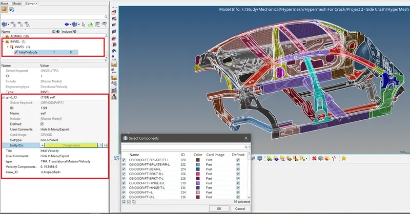
  • Below images shows whether all nodes have been selected or not which can be reviewed by following (INIVEL >> Right Click >> Review) process.

  

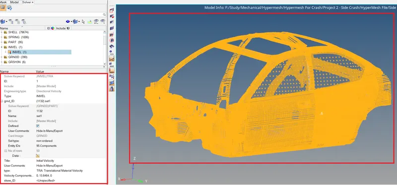
  (10) Sectional Forces

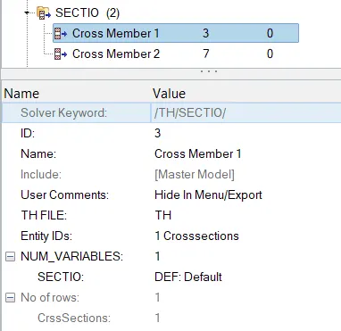
  • The purpose of crashing the car against the rigid wall lies on the concept of sectional force which creates huge impact on the passenger inside the cabin. In this project, section will be created on the different parts of the car model like Cross Members to understand the sectional force on them so that to ensure the safety of passenger inside the cabin.

  #Frame Creation

  • Before creating sectional forces, the frame will be created for components of car model by following (Solver Browser >> Right Click >> FRAME >> MOV) process.

  

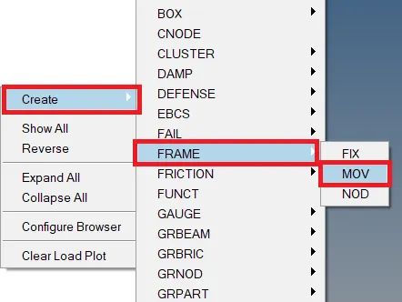
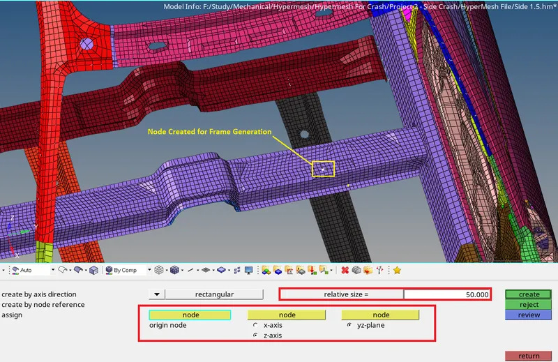
  • Below image shows that local axis coordinate will be created and followed by node creation in origin position, along the z -axis and y-z plane with relative size of 50mm to get picture clearly.

  

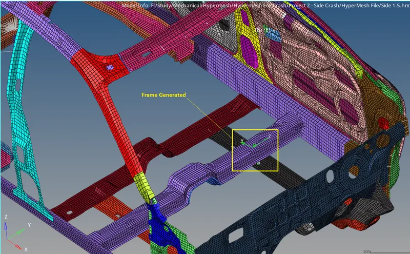
  • Below images shows frame created for the Cross Member 1 and now sectional force will generated for it.

  

  • The section will be created for components of car model by following (Solver Browser >> Right Click >> SECT >> SECT) process.
  • For Cross Member, local coordinate axis of that particular component will be selected by FRAME_ID with delta T of 0.1 and alpha of 0.67.

  

  

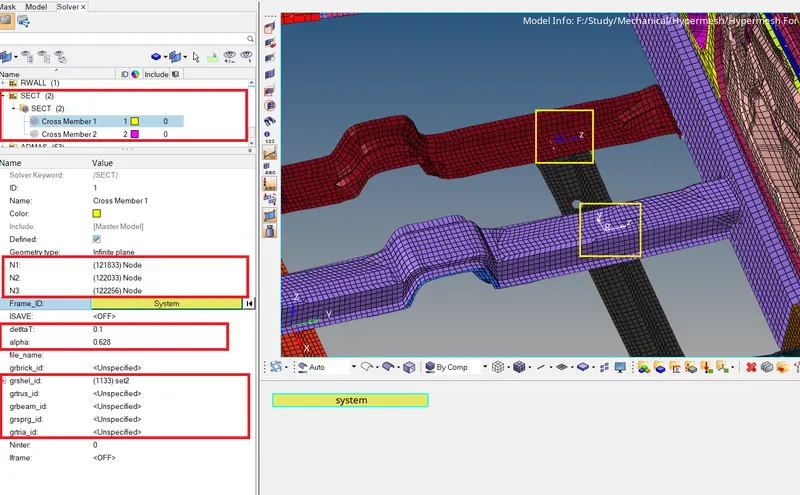
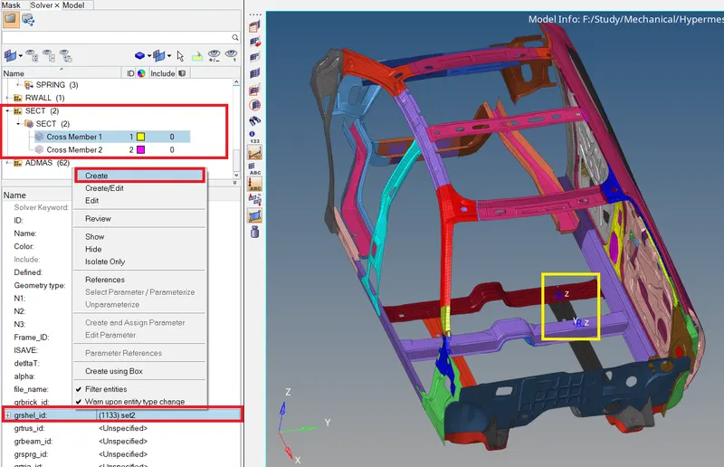
  • Inside grshel_id, particular elements will be selected with specified three nodes aligned to each other on the Cross Member.

  

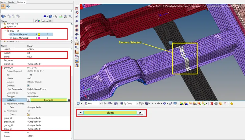
  • Below image shows that sectional force created for the Cross Members of the car model.

  

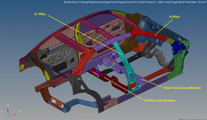
  (12) Intrusion Spring

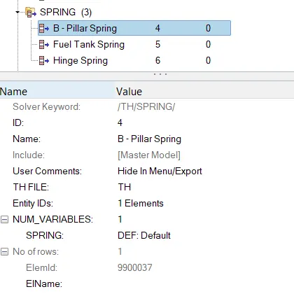
  • Spring elements is created to understand intrusion which means how the forces are coming inside the cabin during deformation. It is opened by following (1D >> springs) process.

  

  

  

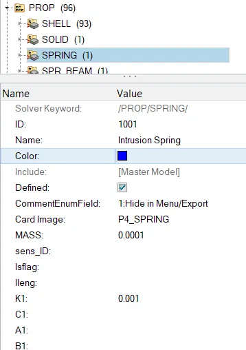
  • After creating spring elements, properties will be applied to them with mass of 0.0001 kg and stiffness of 0.001 kg/mm.

  

  (13) Peak Velocity at Inner Node of Car Door

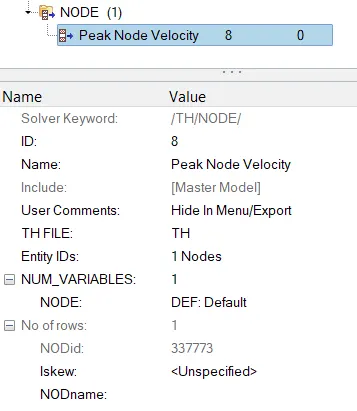
  • The node will be created on the inner portion of car door by following (Solver>>TH>>NODE>>Locates at Inner Node of Car Model) process.

  

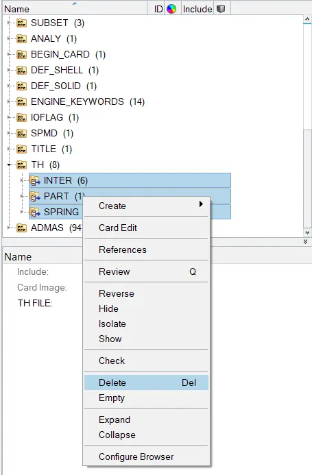
  (14) Delete TH cards create new TH cards

  • Deleting all unnecessary Time History files already present when file imported in the HyperMesh.
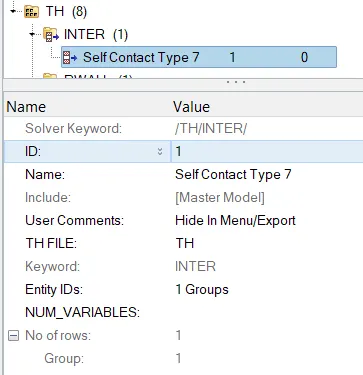
  • Creating Time History files for the operations done above for Node, Type 7, RWALL, and all components sectional forces by following (Solver Browser >> Right Click >> TH >>INTER >>NODE>> RWALL >> SECTIO >> SPRING) process.

  

  

  

  (15) Edit Cards

  • DT Cards
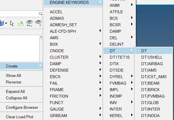
  • DT cards will be created by following (Solver Browser >> Right Click >> Create >> ENGINE KEYWORDS >> DT).
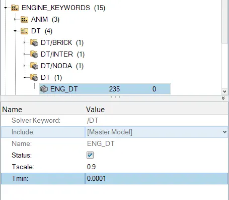
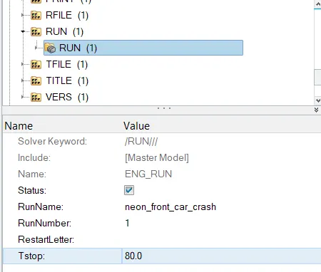
  • The time tolerance for stop criteria of 0.9 and minimum time step of 0.0001 will be provided.

  

  • RUN Cards
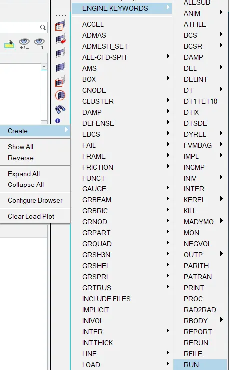
  • Run cards will be created by following (Solver Browser >> Right Click >> Create >> ENGINE KEYWORDS >> RUN) and the final time run of 80ms will be provided.

  

  (16) Model Checker

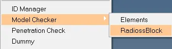
  • After editing cards required for the simulation of car model, error will be checked if any present or mistakes done from the user side for leaving essential values or operation to be performed before running the simulation of car model. It is achieved by following (Model Checker >> Radioss Block) process.

  

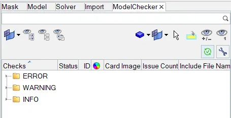
  • Run check on the right side of model checker window frame will be selected in order to run operation to check where the error present inside the model or mistaken done from the instructor side.

  

  

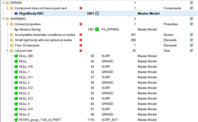
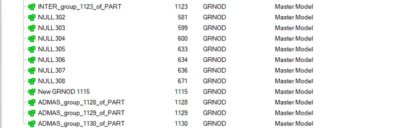
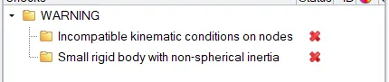
  • After running the operation to check error, now whatever the error present inside the model will be inspected and rectified it according to the conditions. But if errors sticked hardly and unable to remove it from the operation, it will be automatically removed by Auto correct option present at the right side of model checker window frame.
  • Now necessary errors which are creating major problem for running simulation of car model has been removed. Other errors and warnings hardly creating huge impact which will be directly ignored by the instructor. The model checker indicates quality of simulation will be great for the car model.

  

  17) Vehicle Simulation Setup

  • Radioss options will be opened by following (Analysis >> Radioss) process. In Radioss option, file will be saved in desired folder with desired file named as ‘001.out’ which gives energy, mass error and other important properties.
  • The expert options, run options, run number will be maintained as all, analysis, 1 and other option as -nt 4 throughout the base simulation.

  

• • After completing the simulation,the radioss will pop up a solver window stating Radioss Job Completed which indicates the simulation has been completed.
  • Here the number of animation steps obtained are shown in below Figure 97.

  

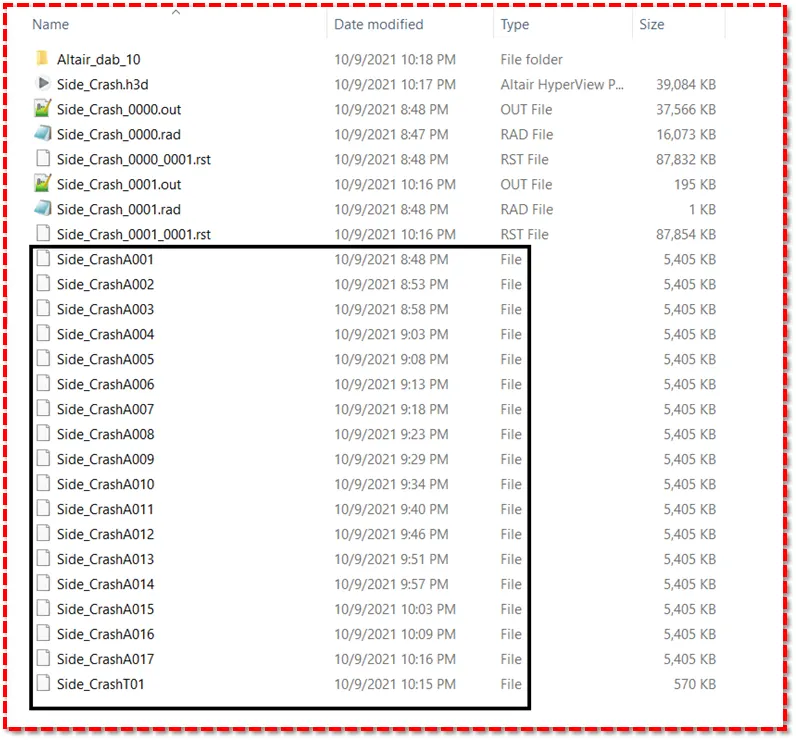
  Figure 97-Animation Files Obtained.

  • Now go and open the 00001.out file with notepad.
  • The obtained values for Energy Error,Mass Error,Internal Energy Error,Kinetic Energy Error and Contact Energy Error has been shown in below Figure 98.

  

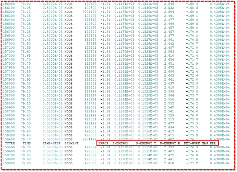
  Figure 98-Obtained values for Energy Error,Mass Error,Internal Energy Error,Kinetic Energy Error and Contact Energy Error.

  • The time taken to complete the simulation and the elapsed time is shown in below Figure 99.

  

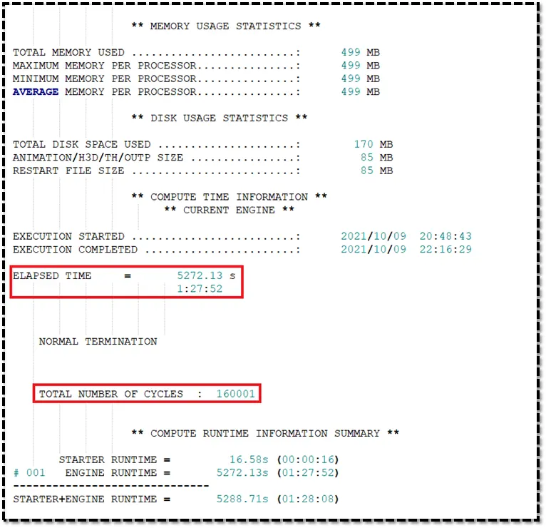
  Figure 99-Time Taken to Copmlete the Simulation and Elapsed Time.

  Phase 12-Post Processing :

  1) Review the Simulation using -HyperView.

  2) Plot the graphs using -Hypergraph 2D.

  1) Review the Simulation using HyperView :

  • Hyperview allows for loading and viewing result files obtained from several sources.
  • Based on the solver type of the files and the results you would like to visualize and analyze,there are differnt ways to load the input deck and their corresponding results into hyperview.
  • First to begin the postprocessing in the Hypermesh,Split the Screen as shown in below Figure 100.
  • Import the animation file .h3d into the hyperview.

  

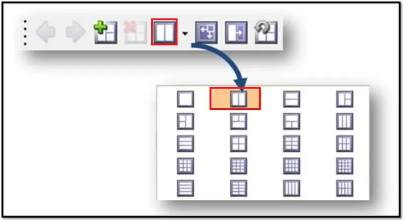
  Figure 100-Splitting the Screen.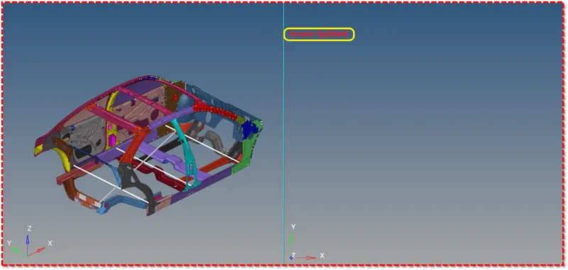

  

  Figure 101-Screen Splitted into Two.

  • And then activate the Client HyperView

  

  Figure 102-HyperView Panel.

  • To access the load model panel
  • Select Load Model Button from the HyperView Panel and open .h3d file as shown in below Figure 103.

  

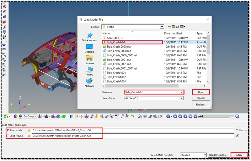
  Figure 103-Opening .h3d File.

  

  Figure 104-Model Loaded.

  • After loading the model into hyperview,It will be represented as shown in below Figure 105.

  

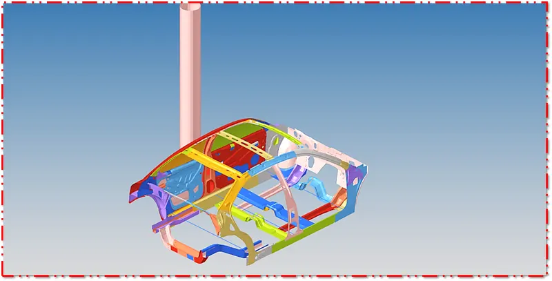
  Figure 105-Model Imported into HyperView.

  • After importing the .h3d file into the GUI,Enable the contour.
  • The contour tool create contour plots of a model graphically visualize the analysis results.
  • To enable contour,Go to Results ToolBar >> Contour .

  

  Figure 106-Contour Panel.

  • Now switch to the Von Misses Stress in result type and select the component,select the averaging method as simple and then click apply as shown in below Figure 107.

  

  Figure 107-Selecting the Paremeters in Contour Panel.

  • After applying ,Run the Simulation,The Simulation animation in terms of Elements,Von Misses Stress and Displacement is shown in below Figure 108,109 and 110.

  

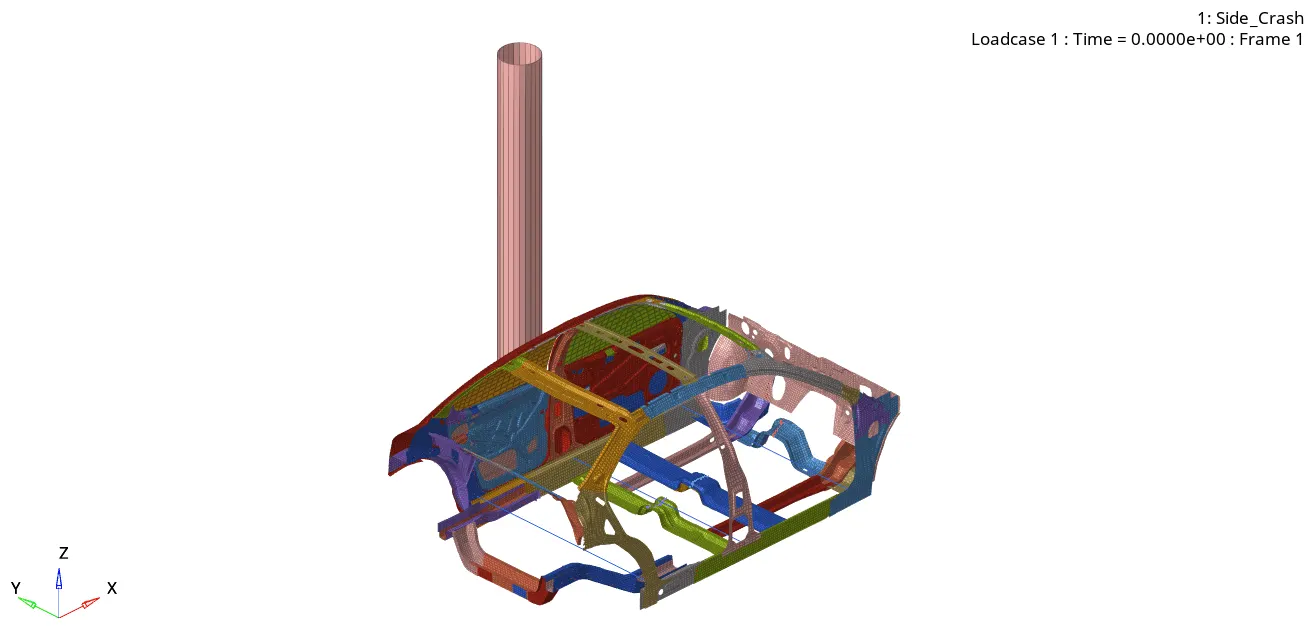
  Figure 108-In Terms of Elements Animation.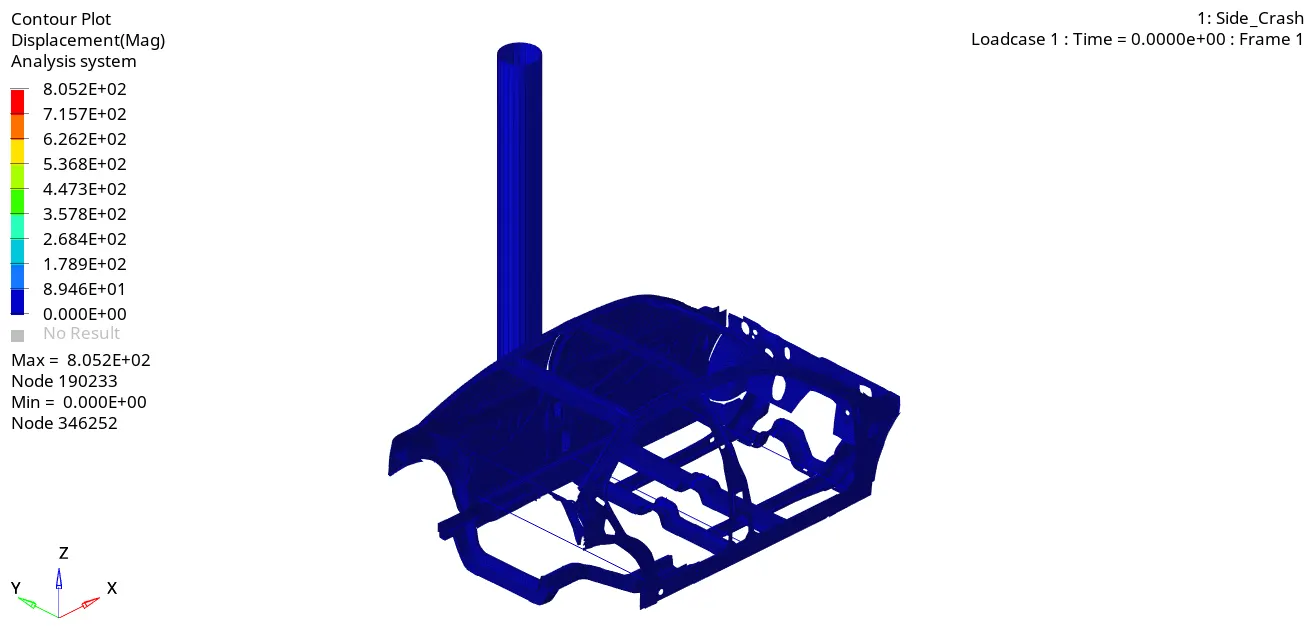

  

  Figure 109-Displacement Simulation Animation.

  • Here the contour plot displays the displacement of each node of the BIW model of a car in a GUI.
  • Displacements are computed with respect to the global co-ordinate system.
  • As the model crashes into the rigid pole,the deformation occurs to each nodes and the nodes gets displaced from their initial position.
  • During the simulation,maximum displacement occured at node 190233 which is shown in above Figure 113.

  

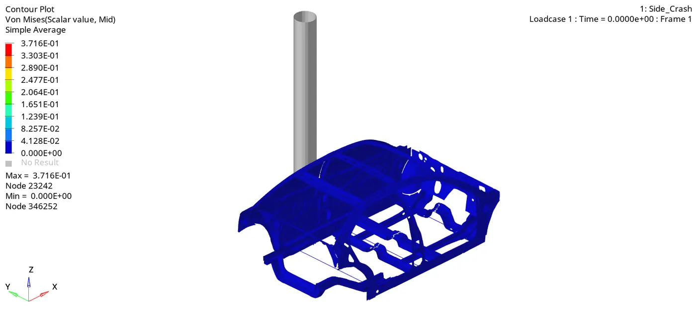
  Figure 110-Von Misses Stress Simulation Animation.

  • Here the contour plot gives the stress induced at each node in the BIW model of the car.
  • As the model crashes,internal stress is developed in the model due to the material behaviour.
  • During this simulation,The maximum stress developed at each node is 23242 which is shown in above Figure 110.

  Check for the Intrusions :

  • After running the simulation,We have to check for the intrusions.
  • Note :The allowable intrusion is 15 cm.
  • To check for the intrusion,Measure the distance between the springs where we created.
  • To measure,Go to Measure tool which is shown in below Figure 111 from HyperView and select the end node of the springs to know the distance between them,which is shown in below Figure 112 and 113.

  

  Figure 111-Measure Tool.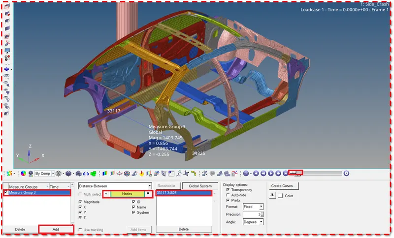

  

  Figure 112-Measuring the Intrusion at Initial Position.

  • After defining the nodes at the end of the spring at the initial position before the collision,The magnitude for the spring is 1403.745 mm.

  

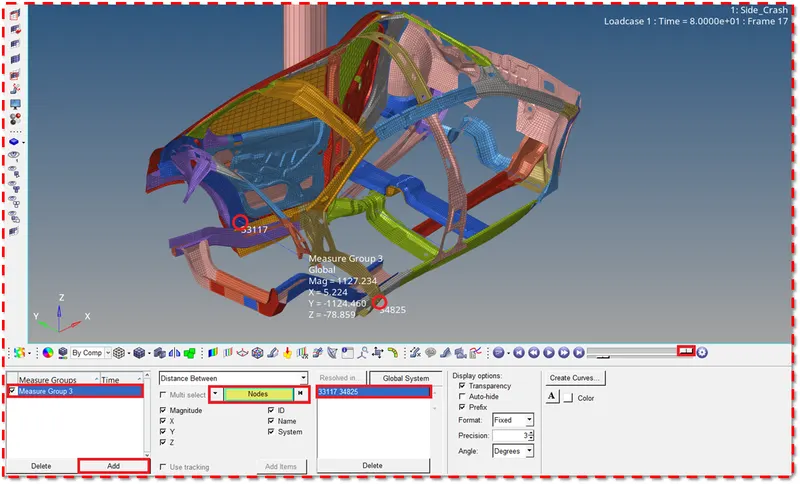
  Figure 113-Measuring the Intrusion After Collision.

  • After defining the nodes at the end of the spring after the collision,The magnitude for the spring is 1127.234 mm.

  Intusion at Fuel Tank Region :

  

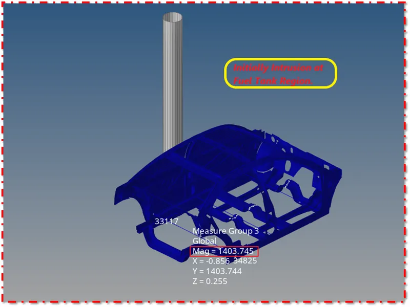
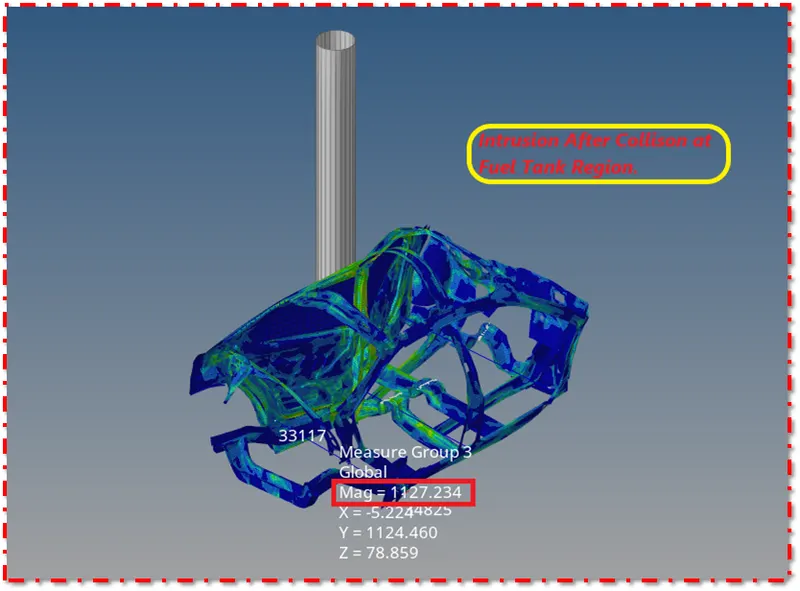
  Figure 114-Intrusion at Fuel Tank Region.

  • Intrusion [Spring] at Fuel Tank Region is 1403.745-1127.234 = 276.511 mm.

  Intusion at B-Pillar Region :

  

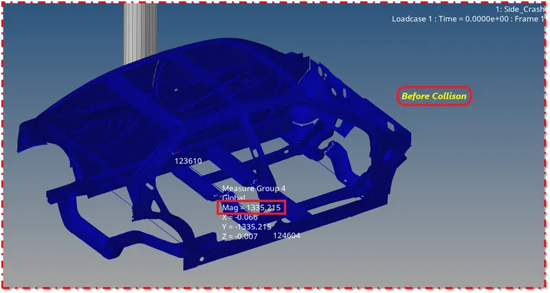
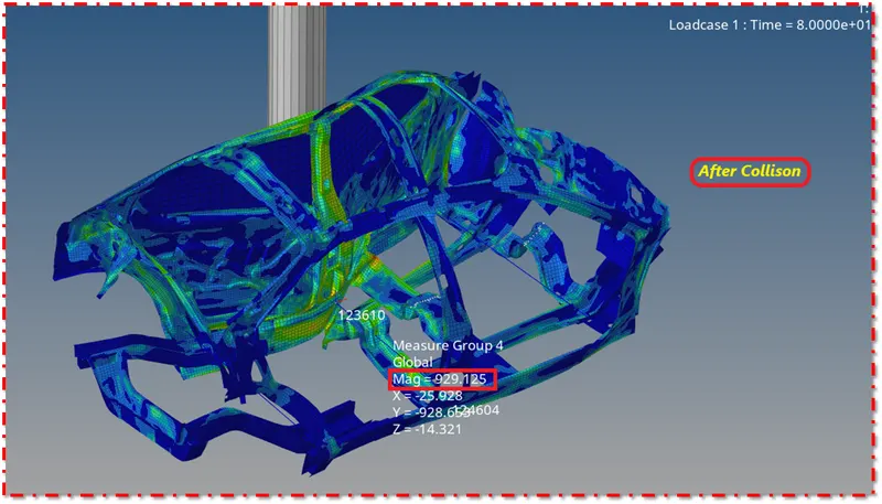
  Figure 115-Intrusion at B-Pillar Region.

  • Intrusion [Spring] at B-Pillar Region is 1335.215-929.125 = 406.09 mm.

  Intusion at Hinge-Pillar Region :

  

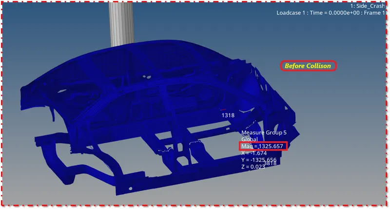
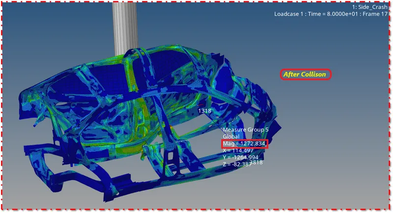
  Figure 116-Intrusion at Hinge-Pillar Region.

  • Intrusion [Spring] at B-Pillar Region is 1325.657-1272.834 = 52.83 mm.

  Plot the graphs using -Hypergraph 2D :

  • Now plot the graphs using Hypergraph 2D,We are plotting the graphs to see what is happening in the rail component.
  • Hypergraph 2D is a powerful data analysis and plotting tool with interfaces to many popular file formats.
  • It is sophisicated math engine capable of processing even the most complex mathematical expressions.
  • Hypergraph 2D combines these features with high quality presentation output and customization capabilities to create a complete data analysis system for any organization.

  

  Figure 117-Switching to Hypergraph 2D.

  • Here switch to the Hypergraph 2D to plot the graphs.
  • To switch,Go to Client Selector >> Choose the Hypergraph 2D as shown in above Figure 117.

  • [Note : Before plotting the graphs,Make sure to split the screen into three or four and then plot the graphs.]

  • The first graph is plotted for the Righ Rail at the created section.

  • To plot the graph,Go to Hypergraph 2D >> Data File >>Frontal_CrashT01 >> Apply.

  Intrusion Graph for Fuel Tank Region :

  • Here the graph is obtained for the Fuel Tank region which is shown in below Figure 118.
  • In the beginning,the length of the spring was 1403.74 mm and after when the car crash the pole,the length of the spring is 1127.23 mm.So the total deflection of the spring is 276.511 mm.

  

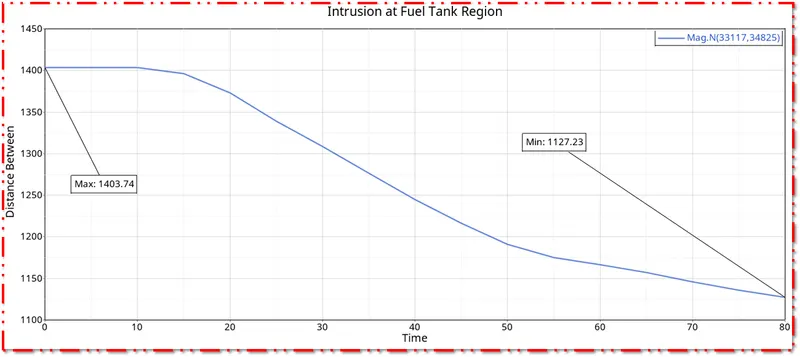
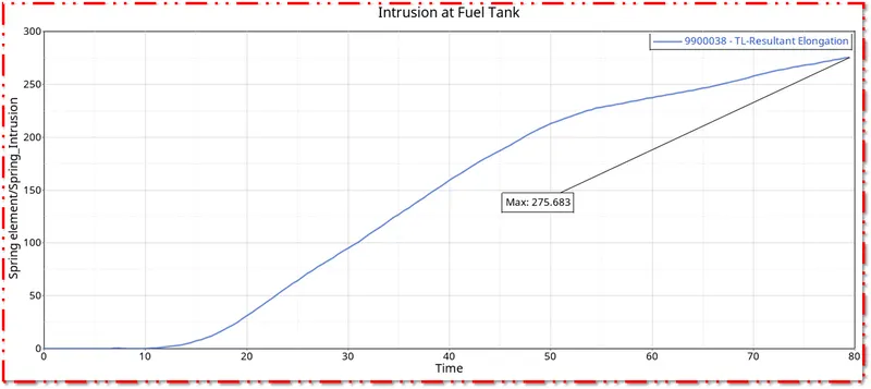
  Figure 118-Intrusion Graph for Fuel Tank Region.

  Intrusion Graph for B-Pillar Region :

  • Here the graph is obtained for the B-Pillar region which is shown in below Figure 119.
  • In the beginning,the length of the spring was 1335.21 mm and after when the car crash the pole,the length of the spring is 929.125 mm.So the total deflection of this spring is 406.09 mm.

  

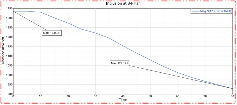
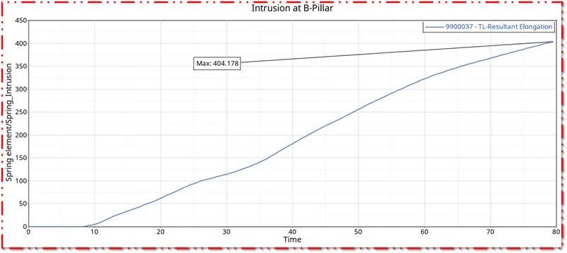
  Figure 119-Intrusion Graph for B-Pillar Region.

  Intrusion Graph for Hinge-Pillar Region :

  • Here the graph is obtained for the Hinge-Pillar region which is shown in below Figure 120.
  • In the beginning,the length of the spring was 1325.66 mm and after when the car crash the pole,the length of the spring is 1272.83 mm.So the total deflection of this spring is 52.83 mm.

  

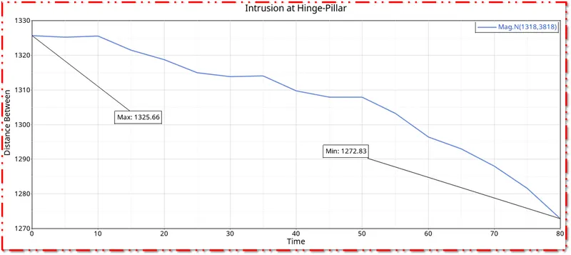
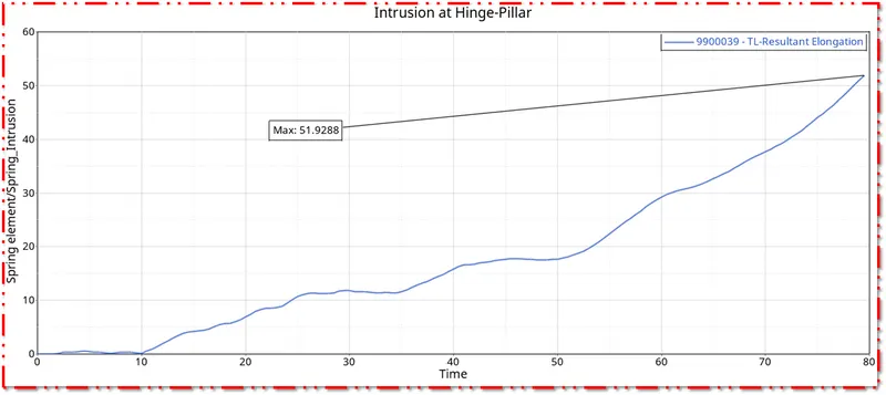
  Figure 120-Intrusion Graph for Hinge-Pillar Region.

  Peak Velocity :

  • The graph obtained for the peak velocity is shown in below Figure 121.

  

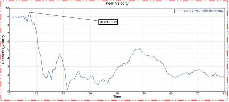
  Figure 121-Peak Velocity Graph.

  • When the car hits the pole,the door will be deformed,So due to the deformation,the inner portion of the door will hit the passengers inside the car and it may cause severe injuries to the passengers.
  • So it is important to calculate the peak velocity at the door region.
  • The peak velocity of the node on the door is 9.51m/s.The graph is in Zig-Zag form,Due to the noise and vibration,When the the car hits the pole.
  • Here the the velocity is starting from peak due to the initial velocity is given and it goes on decreasing,cause the car goes and hits the pole,due to deformation,itse decreasing.
  • We gave the initial velocity as 8.94 m/s,But in the graph,the initial velocity is 9.51 m/s,It's increased little bit,Because due to inertia.

  Interface [TYPE 7] :

  • The graph obtained for the Type 7 - Total Resultant Force Interface is shown in below Figure 122.
  • Here the interfaces curve starts from origin and reaches peak due to collision.
  • And it increases & decreases before it reaches to peak value,Cause there will be a contact forces acting with in the car before collision.

  

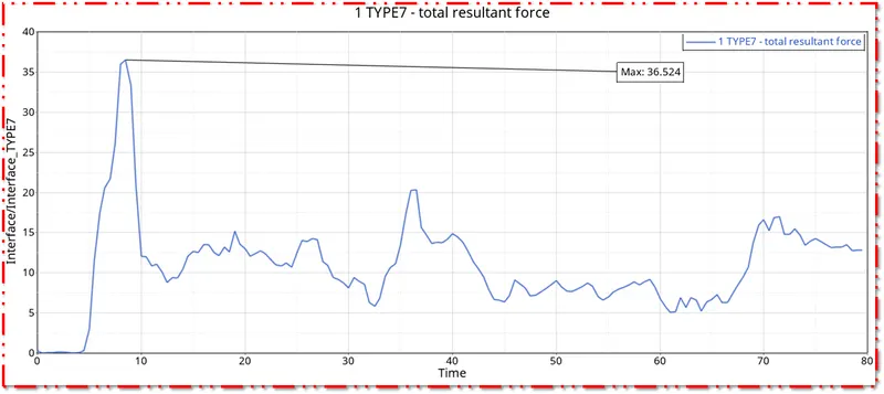
  Figure 122-Type 7 Contact Interface Graph.

  Sectional Force at Cross Member 1 :

  • The graph obtained for the Sectional Force at Cross Member 1 which is shown in below Figure 123.
  • The maximum sectional force on the Cross Member 1 is 3.11726 KN.

  

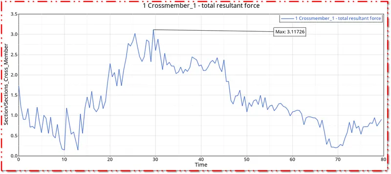
  Figure 123-Sectional Force at Cross Member 1.

  Sectional Force at Cross Member 2 :

  • The graph obtained for the Sectional Force at Cross Member 2 which is shown in below Figure 124.
  • The maximum sectional force on the Cross Member 2 is 4.38827 KN.
  • Here the sectional force is more than the Cross Member 1.

  

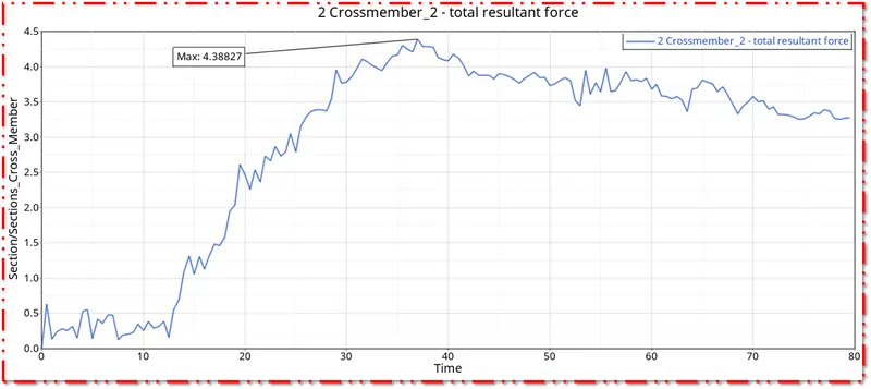
  Figure 124-Sectional Force at Cross Member 2.

  Sectional Force at Cross Member 3 :

  • The graph obtained for the Sectional Force at Cross Member 3 which is shown in below Figure 125.
  • The maximum sectional force on the Cross Member 3 is 0.881435 KN.
  • Here for this Cross Member,the sectional force is very low when compared to the previous two Cross Members.

  

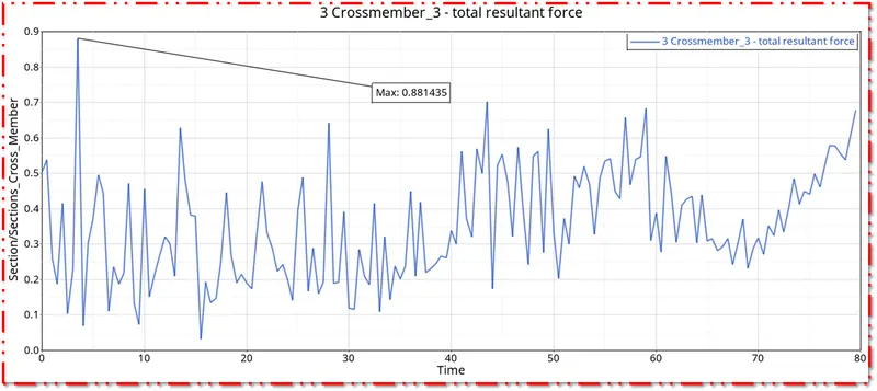
  Figure 125-Sectional Force at Cross Member 3.

  Variation in Sectional Forces :

  

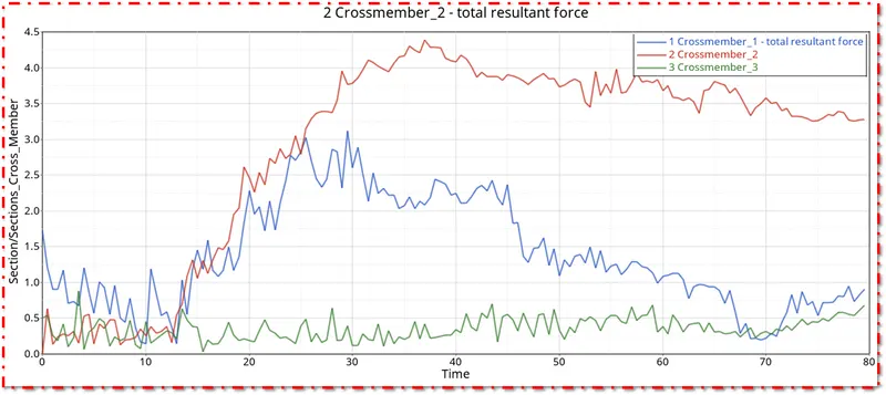
  Figure 126-Variation in Sectional Forces.

  All Energies :

  • All the energies have been plotted which is shown in below Figure 127.

  

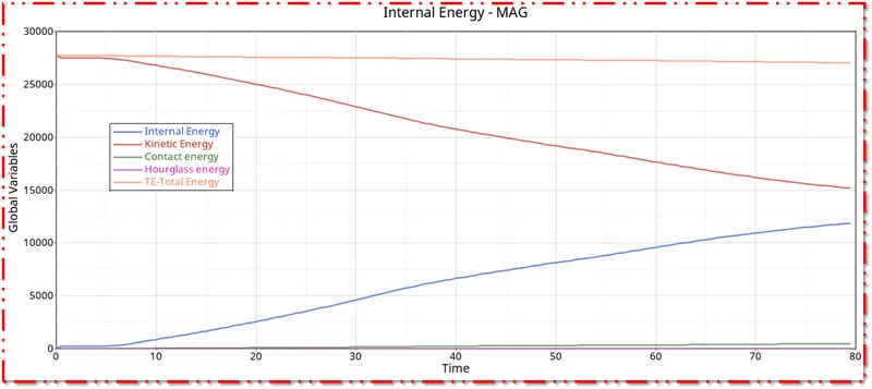
  Figure 127-All Energies Graph.

  Kinetic energy:

  • The graph obtained for kinetic energy is shown in below Figure 128.

  

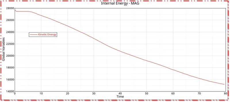
  Figure 128-Kinetic Energy Graph.

  • Kinetic Energy is at peak in the starting,Why because,we have huge mass.
  • Kinetic energy is lower and decreases,why because,there is a velocity applied to the car component,so its getting deformed and the kinetic energy decreases.
  • The kinetic energy will decrease due to the decrease in velocity after the collison,When the car hits the rigid pole. So,the kinetic energy decreases with respect to time.

  Internal Energy :

  • The graph obtained for internal energy is shown in below Figure 129.

  

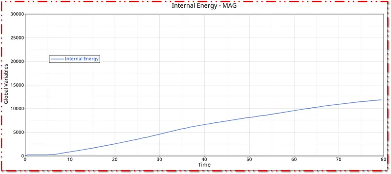
  Figure 129-Internal Energy Graph.

  • The formula for Internal Energy is I.E = Q±">±±W.
  • Here the heat is neglected,Cause there is no heat transfer,We will be having only workdone.
  • W=FxD
  • F=ma
  • Here the internal energy is in Zero,Because there is no deformation initially,So the internal energy is in Zero and starts from Zero and goes on increasing.
  • The internal energy increases because the deformation is happening,there is a displacement,So the internal energy increases,when the displacement or deformation occurs.

  Contact Energy :

  • The graph obtained for Contact Energy is shown in below Figure 130.

  

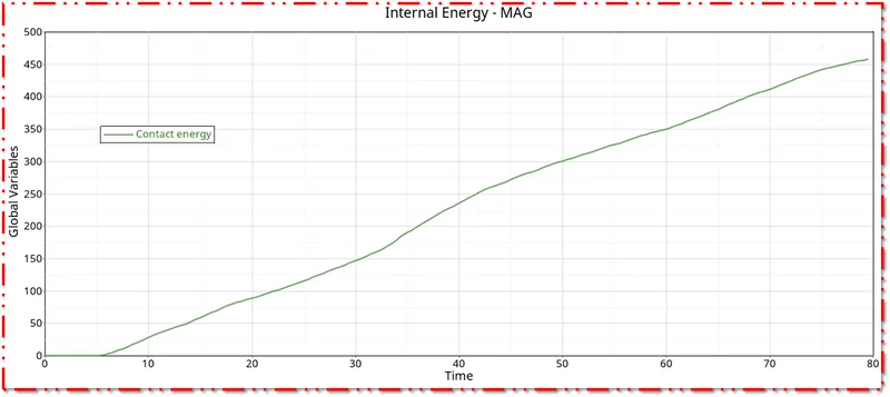
  Figure 130-Contact Energy Graph.

  • Here the contact energy starts from origin,Cause the Car is in intial condition.
  • Intially there is no contact between the Car and Rigid Pole.
  • There is also no deformation intially,But when the car goes and hits on the rigid pole,The contact energy starts increasing.
  • When the deformation or displacement happens to the car,the contact energy increases,cause the car component comes within the contact to the rigid pole.So the contact energy goes on increasing.

  Total Energy :

  • The graph obtained for Total Energy is shown in below Figure 131.

  

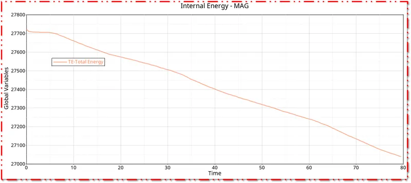
  Figure 131-Total Energy Graph.

  • Total Energy is sum of Kinetic Energy+Contact Energy+Hourglass Energy + Internal Energy.
  • Here total energy starts from higher value,In starting itself its increasing,Why because the total energy is sum of Kinetic Energy+Contact Energy+Hourglass Energy + Internal Energy.
  • All energies are in initial condition except kinetic energy,So kinetic energy is only there
  • Total Energy=Kinetic Energy+0+0+0.
  • Kinetic enrgy is directly proprtional to the total energy.
  • So the total energy is increasing in the beginning.
  • Due to -1.8% of energy error,the total energy is decreasing.

  

  Figure 132-Energy Error.

  Hourglass Energy :

  • The graph obtained for Hourglass Energy is shown in below Figure 133.

  

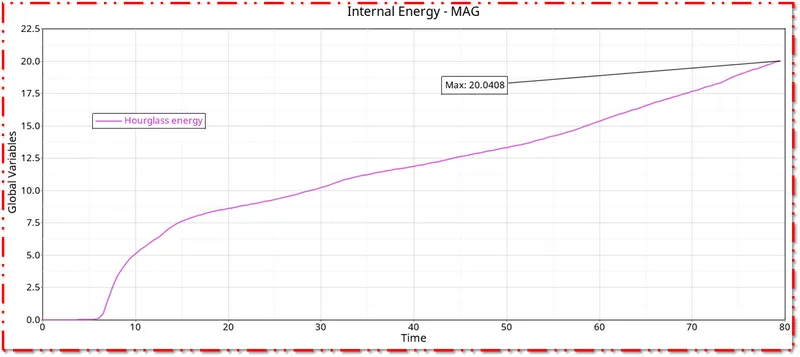
  Figure 133-Energy Error.

  [Note : Hourglass Energy should be less than 5% of Internal Energy.]

  • Here the hourglass energy is less than 5% of internal energy,So it is fine.

  Final Image :

  

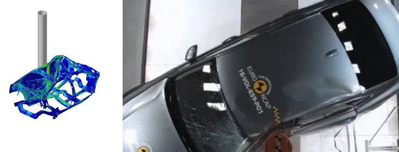
  Figure 134-Final Image.

  • Saftey Standards] 214.

    OBSERVATION:

    There are two types of side pole crash tests are analyzed, 90degree and 75degree sidepole crash. The vehicle that is subjected for the impact is offsetted 15degree in counterclockwise direction in impact's reference line.For a 90degree pole test the vehicle is set perpendicular to the pole and subjected to the crash.

    For 90degree and 75degree crashes the Head Injury Criteria(HIC) and the thorax injury criteria are studied in the crash. From the standards we follow,the results tells us that the 90degree pole test is more reliable than the 75degree pole test. The main advantage of the 90degree pole test is it is common in the real world crash test.

    The 75degree pole test is used only for the observation on opening of the airbag during the crash occured in the Bpillar in the sidepole crash.

    The simulation for the sidepole crash is done for the deformation of the underbody structures. The intrusions and the cross-sectional forces occurs on both the test are compared.

    RESULTS:

    The simulation have been run for the 90degree and the 75degree sidepole crash test is analysed and I go through the crash standards FMVSS and learned about the loadpath, intrusions and the crash parametres used.