Assignment 7

FAST RUNNING MODEL IN GT-POWER

FRMs execute much more rapidly than the typical detailed GT-POWER engine model, and are ideal for integrating with other vehicle systems where an accurate and predictive engine plant model is desired and where computational speed is critical.

FRMs adapt to changing conditions (e.g. valve timing, spark/injection timing, turbo lag, external temperature, altitude, cooling system conditions, etc.) without the need to apply non-physical correction factors. Whether studying changes to ambient conditions, or simulating events that are heavily transient in nature, FRMs will maintain the predictive capabilities of a detailed engine model while allowing for the fast computational speeds that are expected when performing drive cycle analysis and other transient-focused simulations.

FRM models are :

• Fully physical (Able to capture in-cylinder pressure P v/s `theta`). FRM is input-based and can capture using predictive-combustion model
• Dynamic &
• Design to run fast (increasing simulation time step size and decreasing number of calculation per time step).

REPORT on TUTORIAL-9 (Building a Fast Running Engine Model (FRM))

Launching and Initial steps:

• Here we convert the detail 4_cylinder turbo-charged gasolne DI engine (with waste-gate controller and semi-predictive intercooler)model below into FRM model within eight steps.

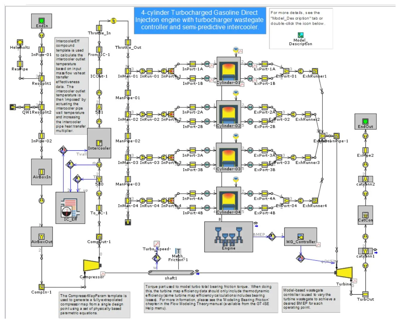
Fig. 1

• Next steps are launching FRM Tags and FRM converter

• Launch FRM Tags i.e. with the high-fidelity engine model open in GT-ISE, go to the Tools tab and click on 'FRM Tags'. The model has already been tagged. We can select the individual subsystem and the parts are getting highlighted on the map.

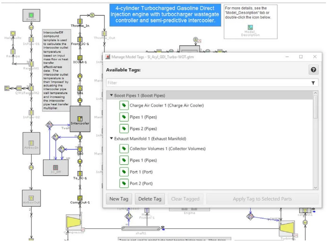
Fig 2.

• Launch the FRM Converter. With the high-fidelity engine model open in GT-ISE, go to the Tools tab and click on 'FRM Converter'. This will prompt to create an FRM Conversion Project.

Major Steps involved :

1. Exhaust Manifold : For high-fidelity models, this is almost always the exhaust manifold where the highest gas velocities occur, which in turn restricts the time step. Hence, this is first taken care of. Basically here the exhuast ports are converted to single volume as can be compared with fig 1.

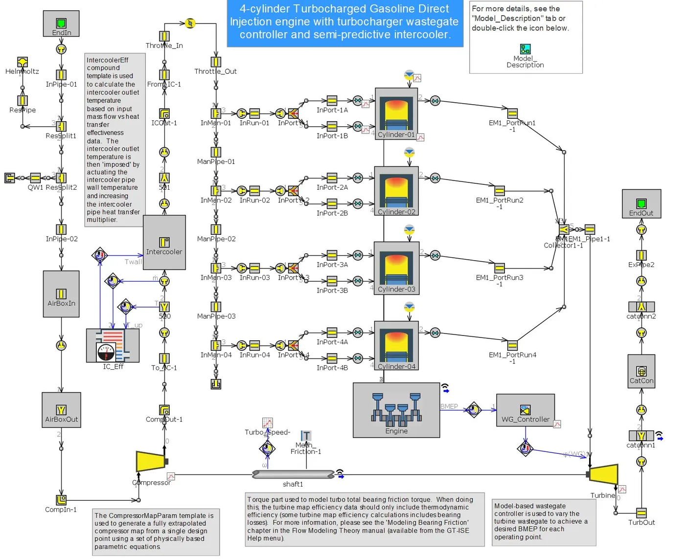
Fig 3.

2. Exhaust Pipes: For the second step of model simplification, the exhaust pipes downstream of the turbine will be simplified. Name the step "Exhaust Pipes". Select Exhaust Pipes 1 from the Tagged Subsystems list. Click on "Simplify for Accuracy" and click "Yes" for the "Delete Part" dialog.

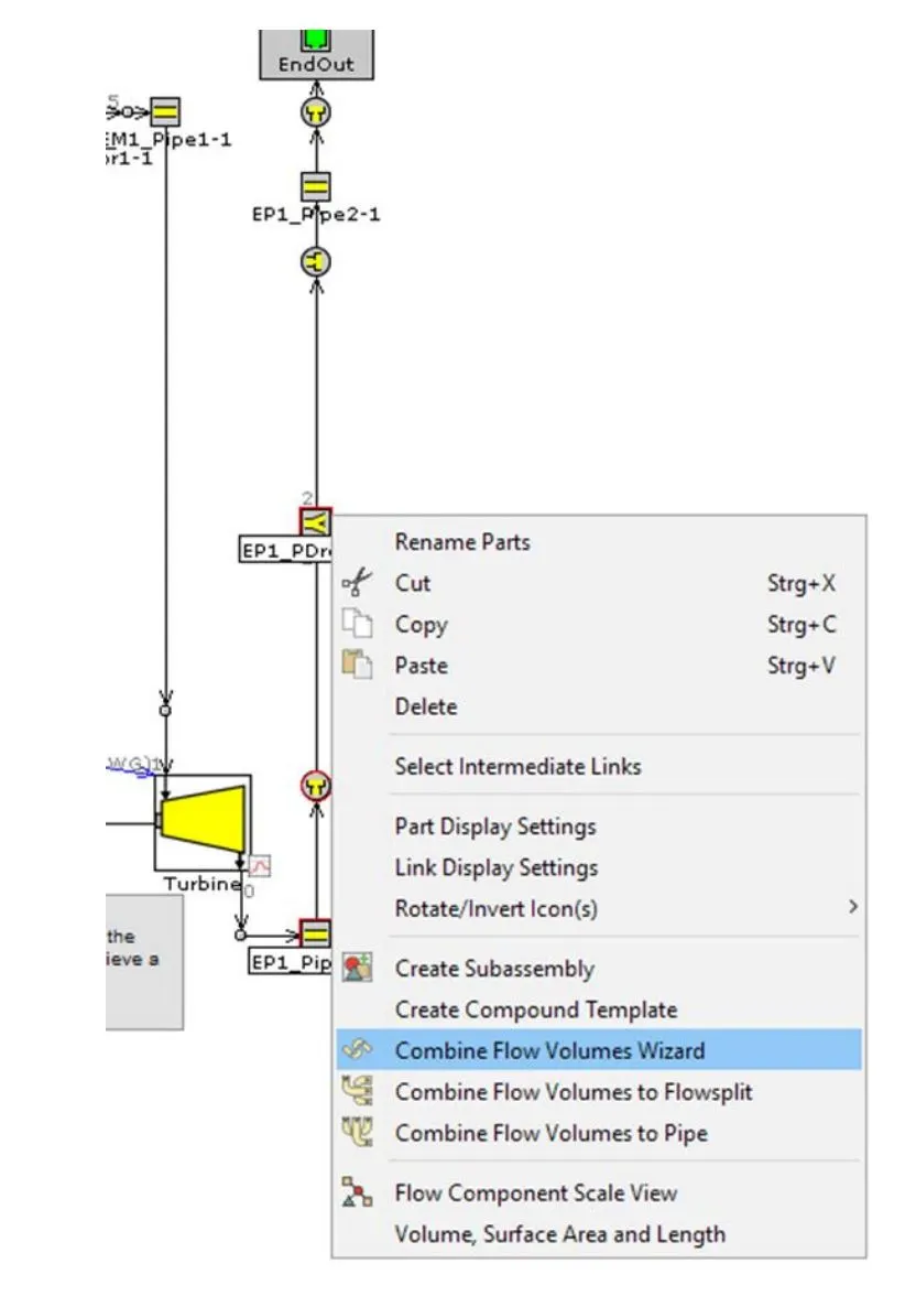
Fig 4.

Once in the Combine Flow Volumes wizard, keep "Combine flow volumes to Flowsplit". Final network is obtained below i.e. the after treatment system is converted to flow-split general templetate

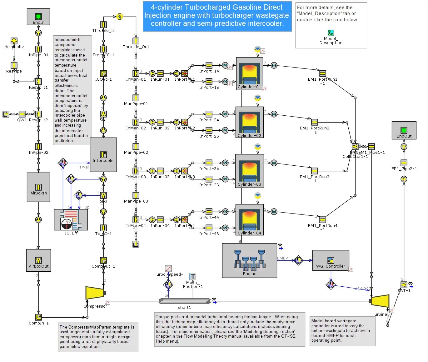
Fig 5.

3. Intake manifold: Name the step "Intake Manifold". Select Intake Manifold 1 from the Tagged Subsystems list. Click on"Simplify for Accuracy". Click "Yes" on the Delete Part dialog; this will be handled later. Collapse the FRM Converter to provide space to work in the model map. Similar to exhaust manifold here the intake system is converted to single volume.

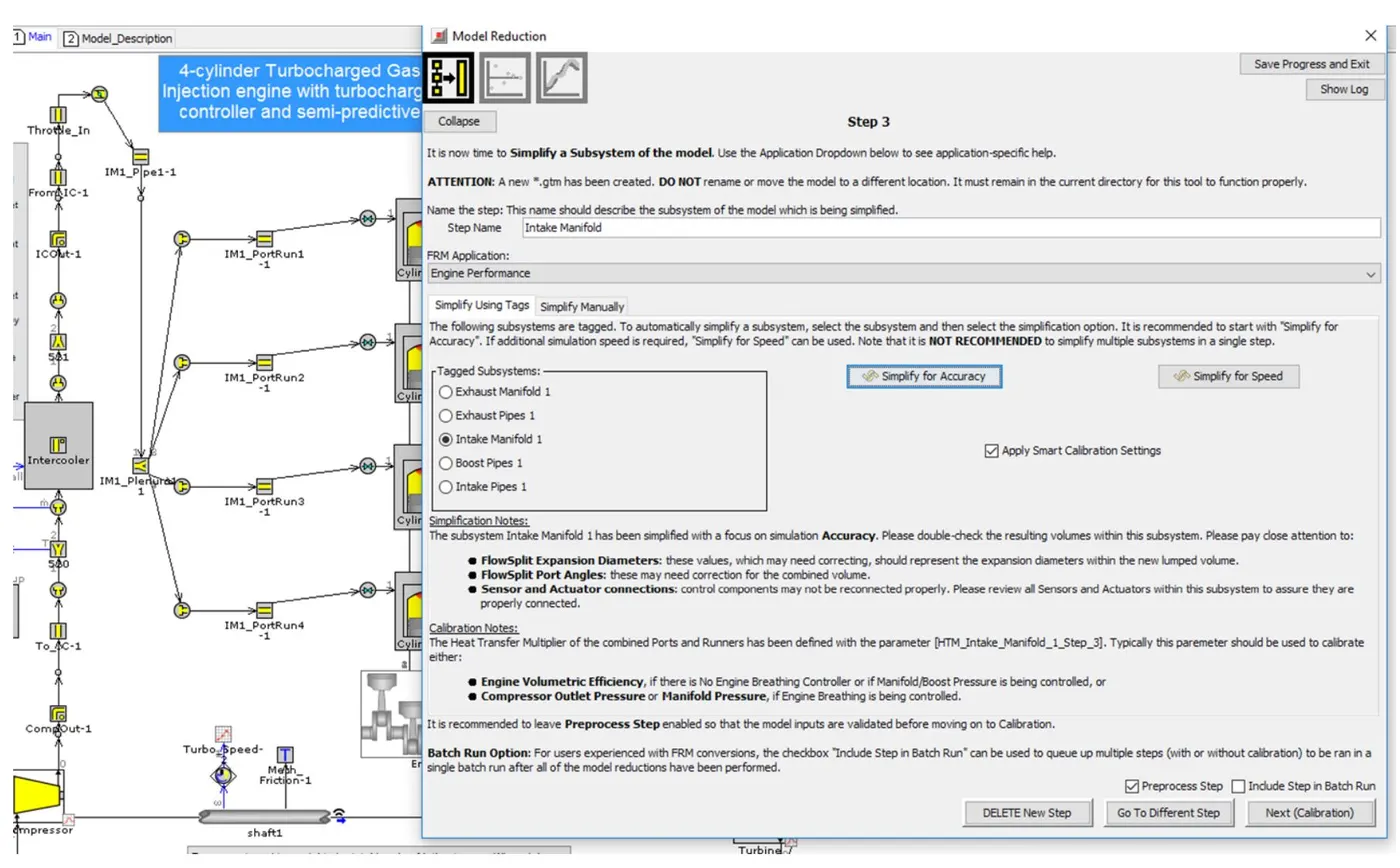
Fig 6.

4. Compressor Outlet pipes: Name the step "Compressor Outlet Pipes". Select Boost Pipes 1 from the Tagged Subsystems list. Click on "Simplify for Accuracy". Collapse the FRM Converter to provide space to work in the model map. This step is quite similar to step 2 i.e. turbine outlet pipes. The Intercooler Diameter will be adjusted in order to maintain compressor outlet pressure.

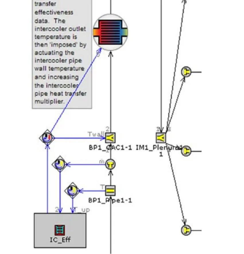
Fig 7.

5. Intake pipes: Environment input to throttle valve input is converted to FRM model

Fig 8. Shows the complex network from end environment to throttle valve

Name the step "Intake Pipes". Select Intake Pipes 1 from the Tagged Subsystems list. Click on "Simplify for Accuracy". Collapse the FRM Converter to provide space to work in the model map. Expand the FRM Converter and click "Next (Set Calibration)" to preprocess the model and continue
to Calibration.In the Calibration page, select Case 1 for calibration. Under "Configure calibration…", change theResponse RLT to the Compressor Massflow-Averaged Inlet Pressure (cmp-pia:Compressor). . Set the lower and upper values of the range for DIA_Intake_Pipes_1_Step_5

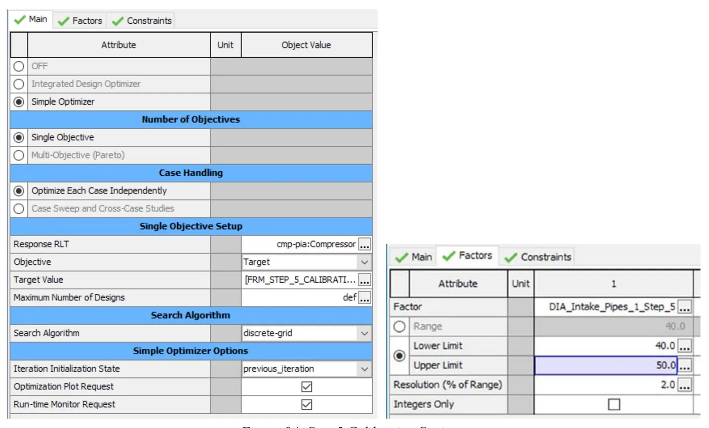
Run the calibration, and once it is finished, click "Next". In the Results page, click "Run Model" to rerun the full set of Cases. Check the model results and assure that they are satisfactory.

Fig 9. Final reduced network of intake pipes

6. Additional Changes :Name the step "Additional Changes". Select Exhaust Manifold 1 from the Tagged Subsystems list. Click on "Simplify for Speed". Basically, this is further simplication for exhaust manifold system.

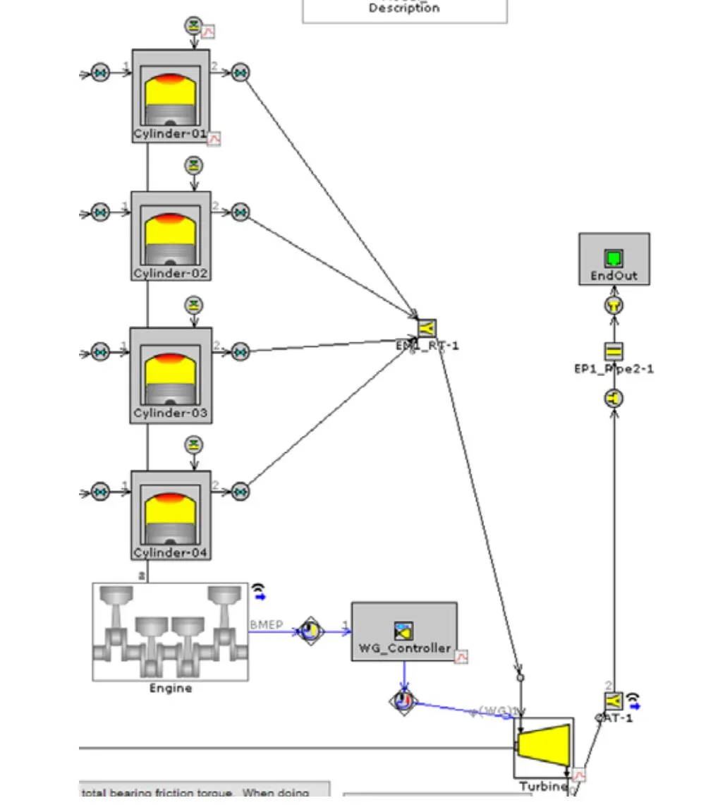
7. Cylinder Slaving : The final simplification to the model will utilize the Cylinder Slaving capability of the EngCylindercomponent. Name the new step "Cylinder Slaving", then collapse the FRM Converter to provide space to work in the model map. A master cylinder a large cylinder in a hydraulic system in which the working fluid is compressed by a piston enabling it to drive one or more slave cylinders. The slave cylinders in a car are used to finish the amplification of the forces from your foot inputs through to the clutch and brakes respectively.

Right-click on any of the EngCylinder parts on the map and choose "Edit Parent Object". Go to the"Advanced" tab and for "Cylinder Slaving Option", select "slave-RT-full-v2018", then click OK. Nowdouble-click on Cylinder-01, go to the "Advanced" tab, and set the Cylinder-01 override value of "CylinderSlaving Option" to "master".

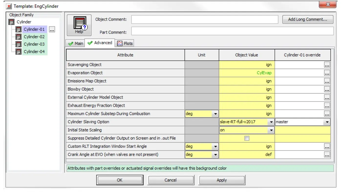
For the full cylinder slaving to function, each Valve must be specified as either an Intake or Exhaust valve. The intake ones start with "IM1_PortRun” and the exhaust ones start with "EM1_PostRun". Expand the FRM Converter and click "Next (Calibration)" to preprocess the model and continue to
Calibration.

8. Real-Time Solver (optional, only available with an RT license) :

Click "Next (Begin Next Step)" in the FRM Converter. Name this new step "Real-Time Solver", thencollapse the FRM Converter. To run with the real-time solver, the license type of the model must bechanged. However, certain templates are not allowed with the real-time solver, and so they must first be removed from the model.

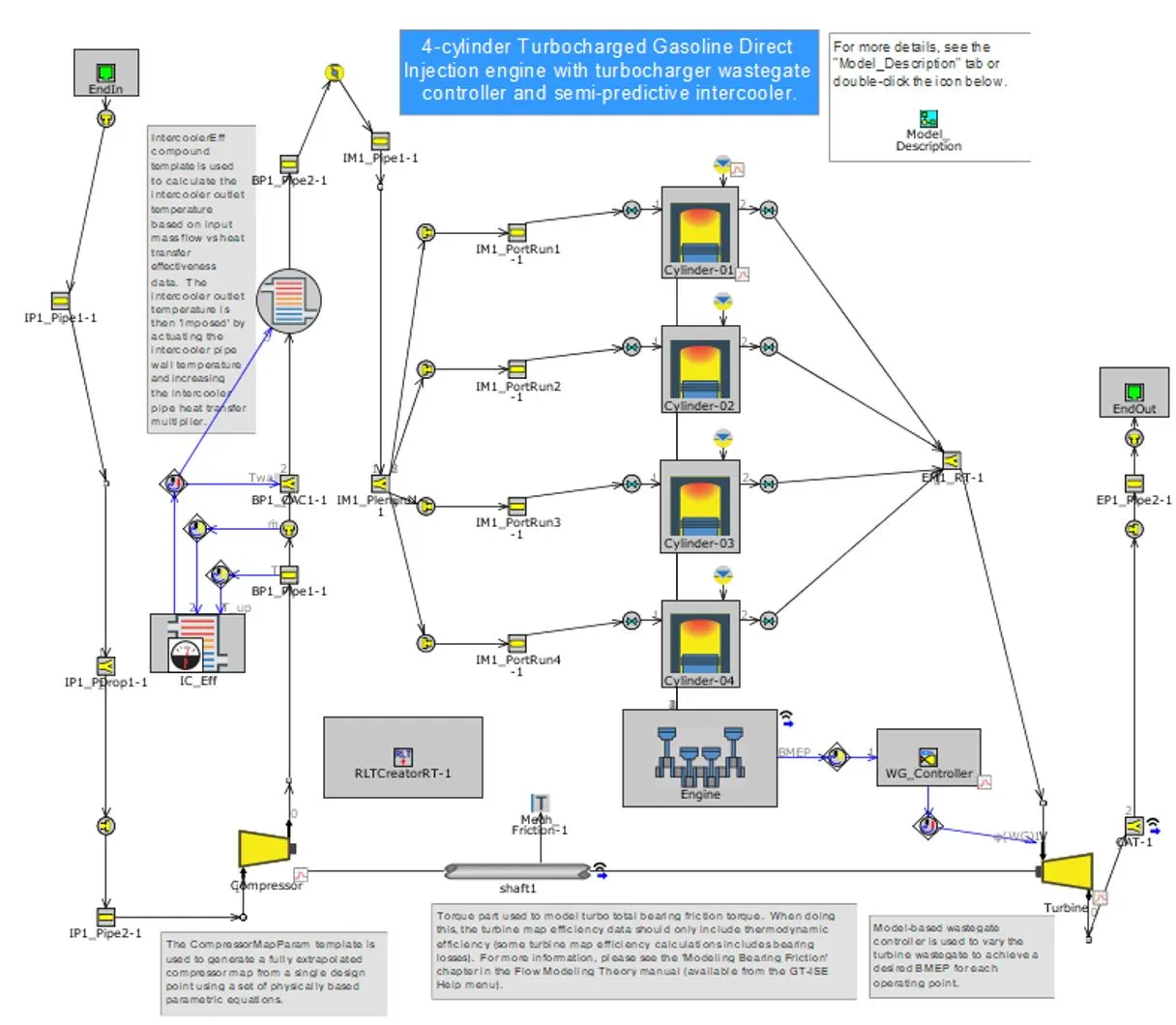
The final network i.e. the detailed model is converted to FRM model using above steps.

FRM MODEL BUILDER (Using FRM builder approach):

Following steps are done for building the FRM model using builiding technique :

• Go to Tools- FRM model builder icon

• Select the CI engine model

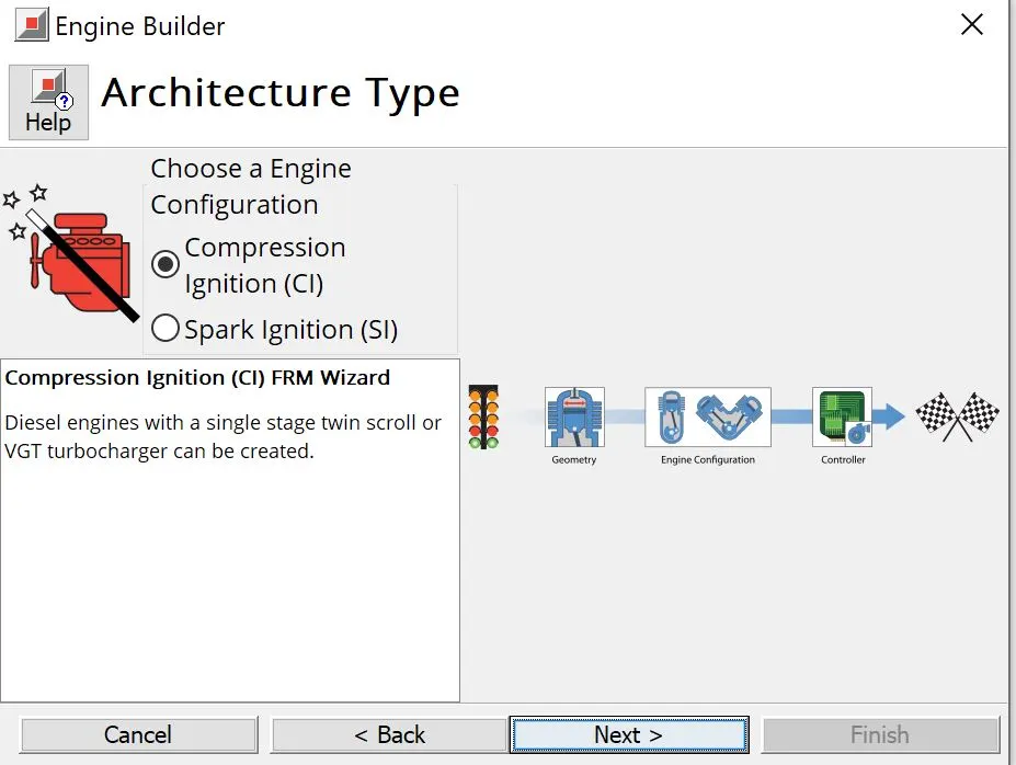
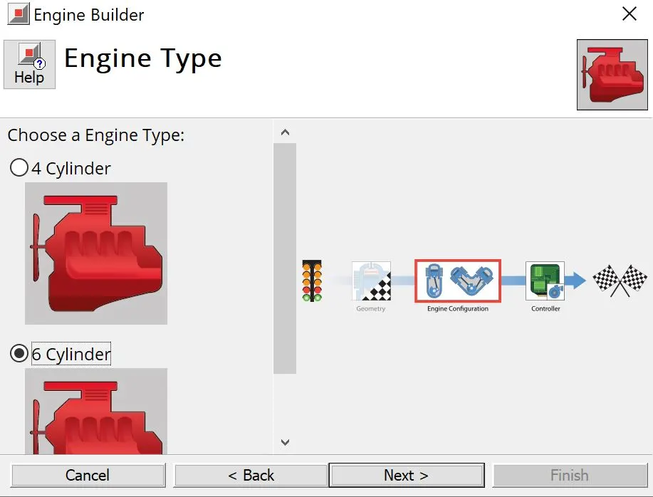
• Select the 6-cylinder engine configuration

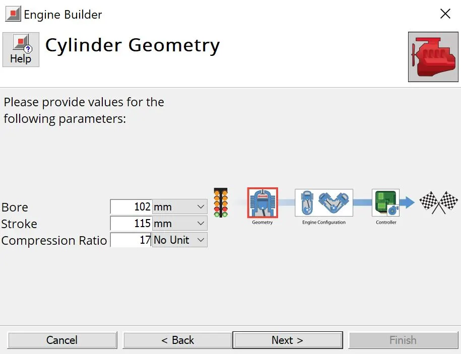
• Give the cylinder geometry details as below :

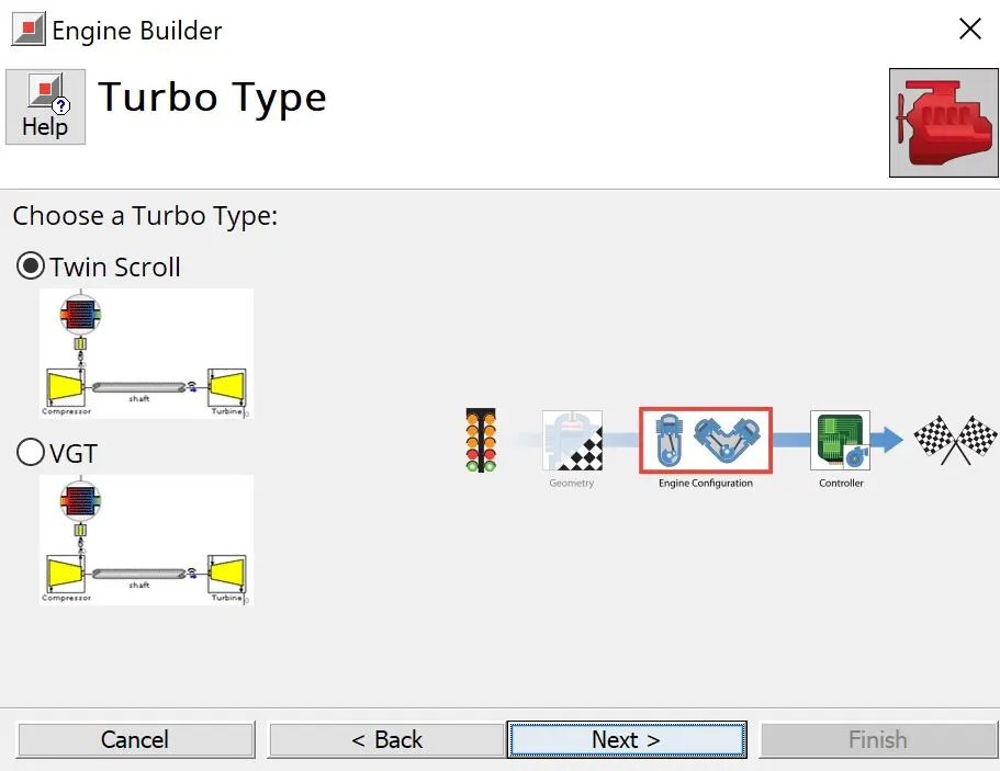
• Select the twin-scroll turbine

• Select GT- suite controller for control-logic type

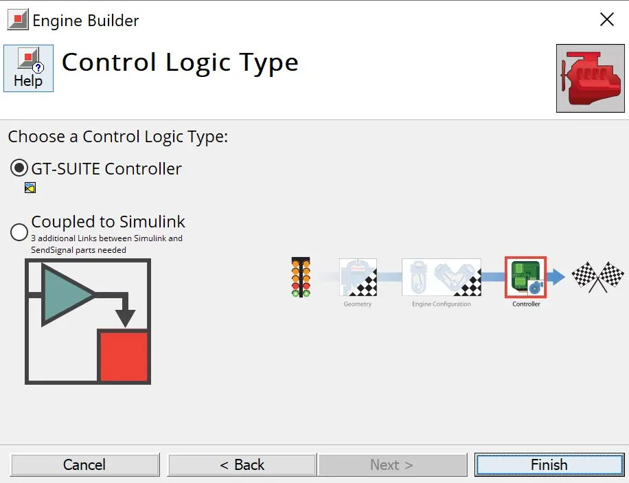
• Select finish and the following model is created

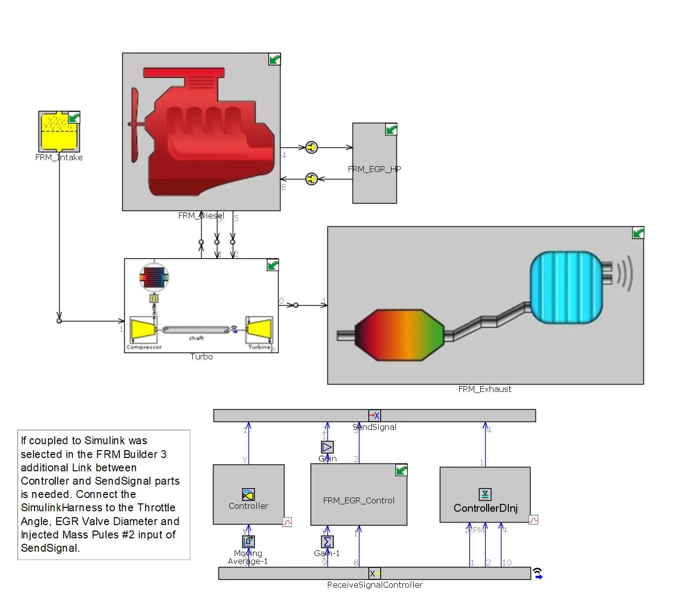
• The following setup is run for 25 cases and we will study each of 8 case just after we see these plots below :

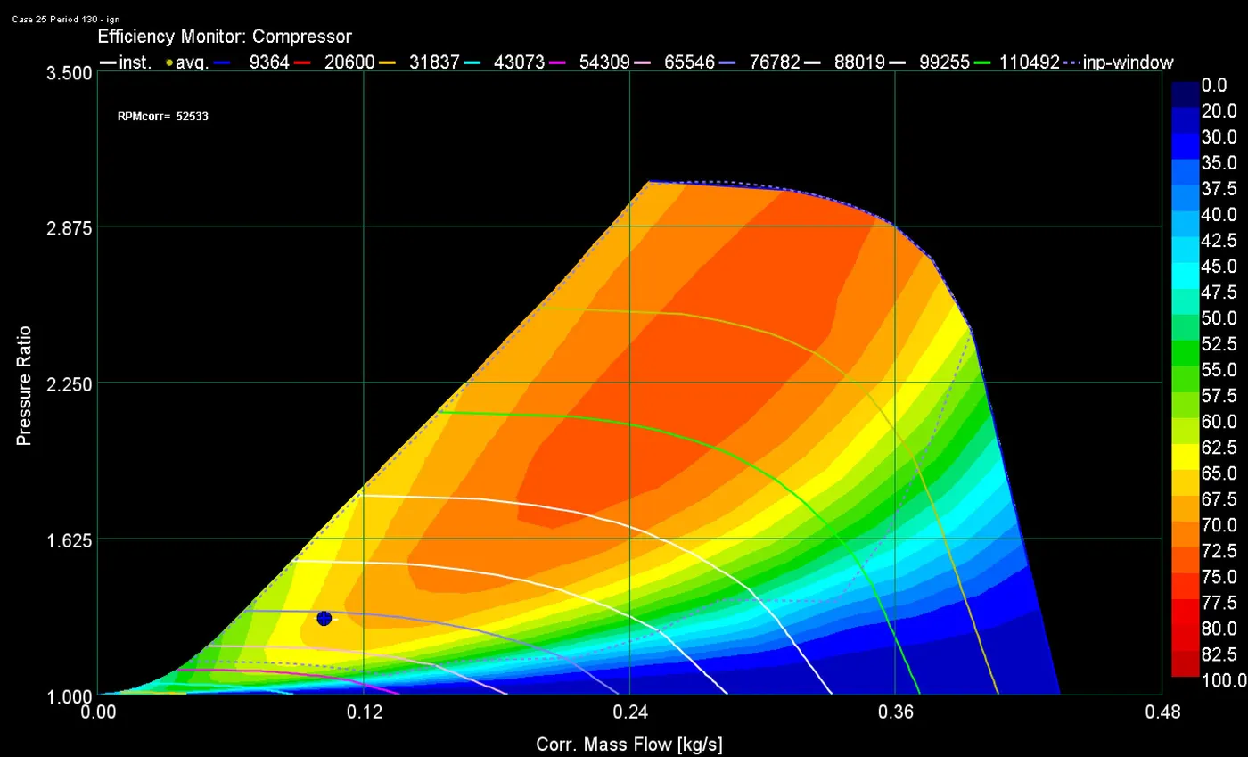
Compressor Efficiency

• The operating points of the compressor are within the limits for 25 cases run and efficiency of compressor in near 70%.

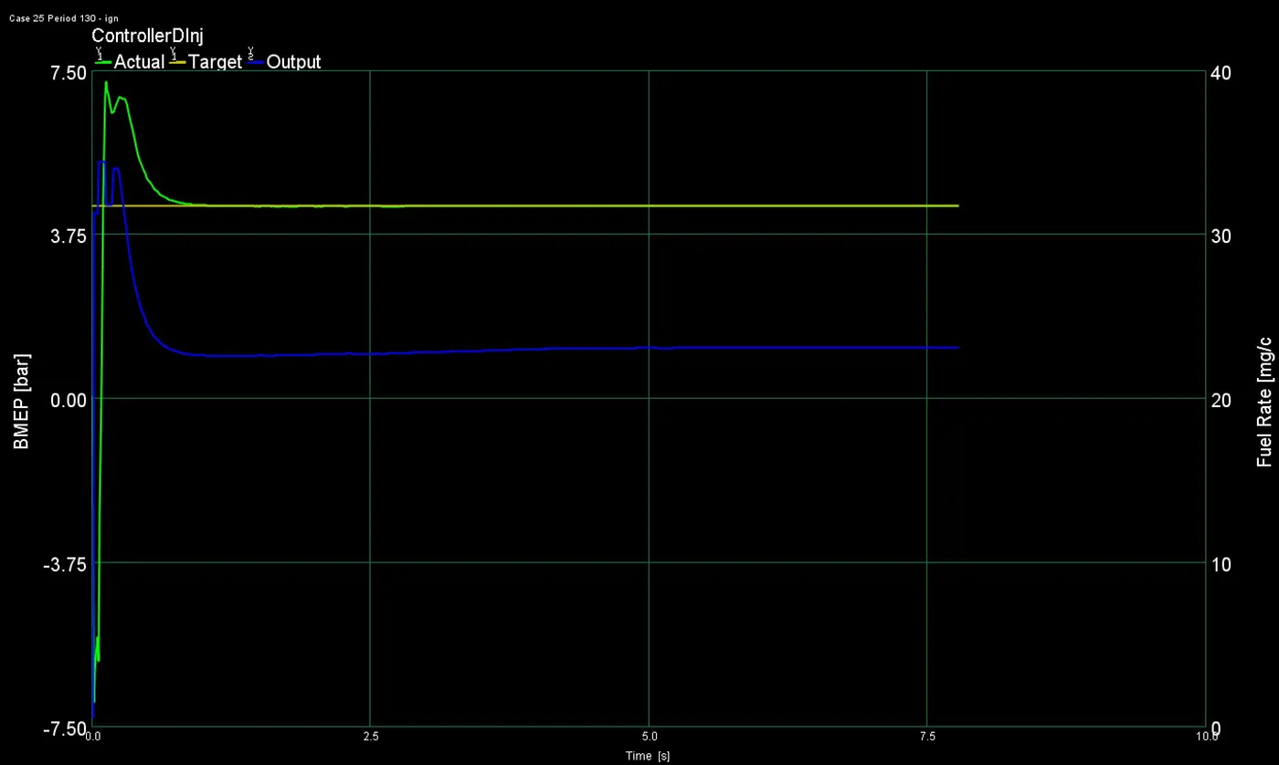
• BMEP targets are achieved and converge quickly

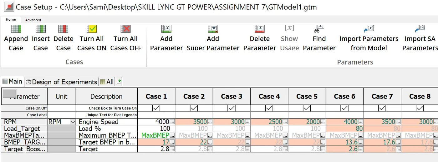
Cases are divided into three sub-cases. Following cases are studied:

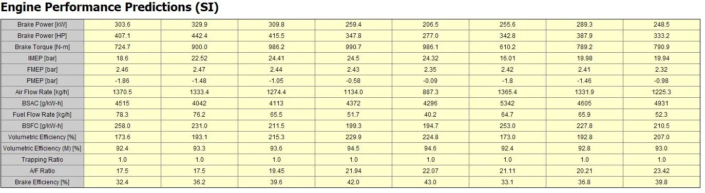
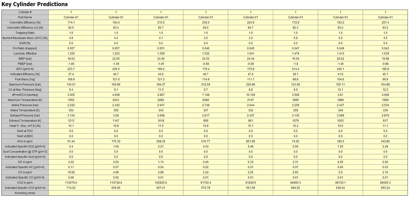
CASES (1-8) :

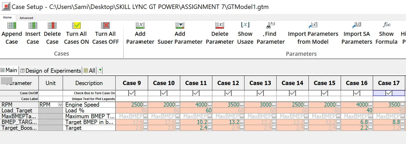
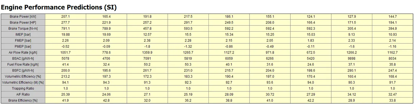
CASES (9-17) :

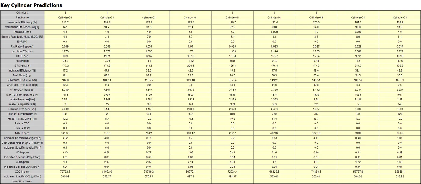
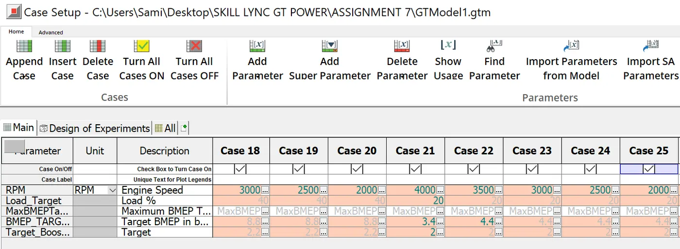
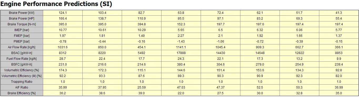
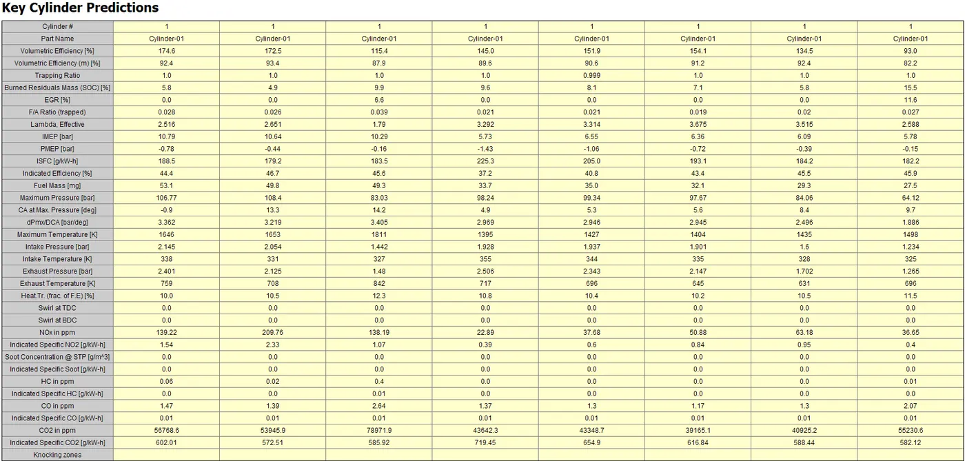
CASES (18-25) :

SUMMARY :

1. Tutorial -9 is explained in step-wise detailment
2. FRM building approach was used to built a 6-cylinder twin-scroll CI engine with GT-type controller.
3. Cases are run at varying 4000-2000 RPM's along with target BMEP's and Boost condition and following is observed.

• A/F ratios increase on increase in boost i.e. due to the air sucked in more and NOx values increases
• Power and Torque values are increased as Target BMEP values are high
• Compressor operating points are within the range limits.