Assignment 7
Assignment 7 Fast Running Model (FRM) Approaches
- AIM:
- Explore the fast-running model using FRM convertor and builder approach.
- OBJECTIVE:
- Explore the FRM Convertor Approach
- Build FRM Model for following configuration using FRM builder approach.
- Bore 102 mm stroke 115 mm CR 17
- No of cylinder 6
- CI engine
- Twin Scroll Turbine
- GT Controller
- Procedure:
Introduction
Fast Running Engine Models are dynamic, fully-physical engine models that are designed specially to run fast. While high-fidelity engine models are commonplace in the engine performance department, they are often too slow running to incorporate into system level models where long transient events may be simulated, or where the simulation model must respond faster than real-time, such as for HiL (Hardware-in-the-Loop) simulations. When simulation speed is of priority, high-fidelity GT-POWER engine models can be simplified into FRMs using a standard conversion process. It is up to the user how far to simplify the model, depending on the accuracy-vs.-runtime requirement.
FRMs are able to achieve such fast run times by two means:
(1) increasing the simulation time step size, and
(2) decreasing the number of calculations per time step.
These two means are often accomplished at the same time by lumping various ow volumes together which will reduce the total number of sub volumes and also allow for a larger time step size by increasing the effective sub volume length (which is responsible for the time step size). In addition to simplifying and combining ow volumes, there are additional solver options that can reduce the number of calculations per time step and, thus, further decrease the run time without changing the time step size.
Some examples of applications that are ideal for FRMs are:
- ECU Modelling (including Hardware in Loop) – where a fast-running and transient-capable engine model is essential for optimizing ECU strategy.
- Engine + Drivetrain/Vehicle – where accurate torque pulsations are key for optimizing drivetrain design and strategy.
- Vehicle Thermal Management modelling, where the engine provides the heat to the cooling system, and the cooling system behaviour feeds back into the engine performance predictions (great for simulating off-ambient conditions)
Explore the FRM Convertor Approach-Tutorial No. 9
Conversion of detailed model to FRM
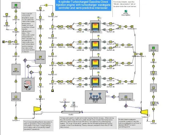
This model is a 4-cylinder 2.0 litre turbocharged Gasoline Direct Injection (GDI) engine. The turbine wastegate is being dynamically controlled in order to target BMEP. A full-load speed sweep is being simulated, from 5000 RPM down to 1000 RPM. A semi-predictive charge air cooler is included such that the outlet temperature is predicted as a function of inlet gas temperature and mass ow rate, coolant temperature, and charge air cooler effectiveness.
Timestep Restricting Parts, Number of Sub-volumes
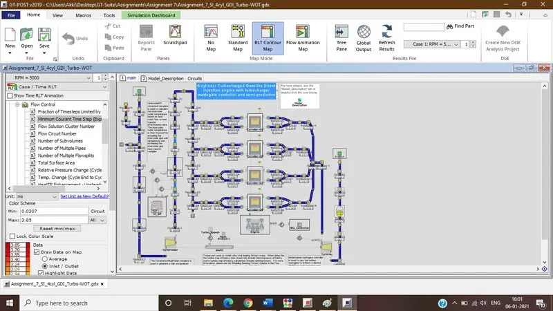
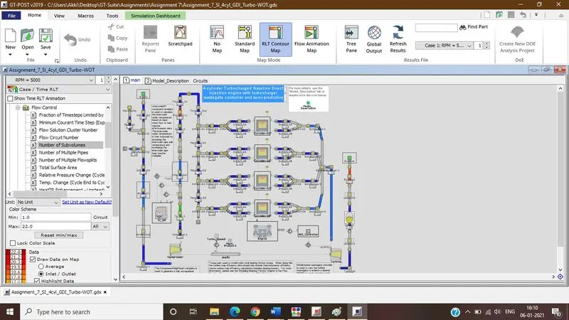
This will give an overview of all parts and the associated courant number. The lower the value, the more likely the part will limit the timestep. This enables the user to determine multiple parts that will limit the timestep.
Another option to determine timestep limiting parts is to select "Fraction of Timesteps Limited by Part" directly above "Minimum Courant Time Step (Explicit Circuits Only)". In contrast to the courant number only parts that limit the time step will be displayed.
Launch FRM Tags
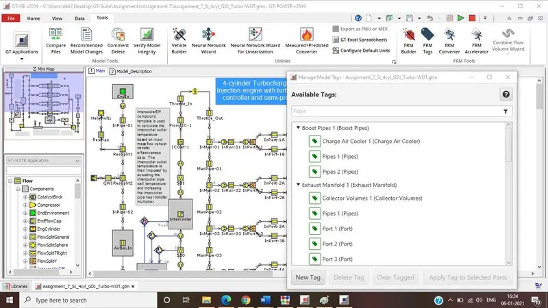
With the high-delity engine model open in GT-ISE, go to the Tools tab and click on 'FRM Tags'. The model has already been tagged. You can select the individual subsystem and the parts are getting highlighted on the map.
Launch the FRM Converter
The GT-SUITE FRM Converter is a tool that will track the FRM Conversion process, organize all model les automatically within subdirectories, and provide result comparisons of key RLTs throughout the conversion process. The process information is stored in a *.frm le which can be saved and reloaded at any time to review the process or to continue where you left off.
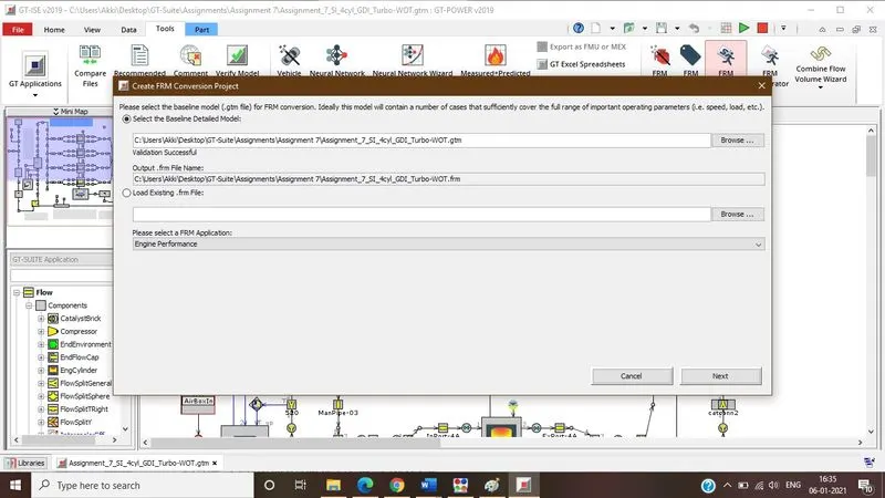
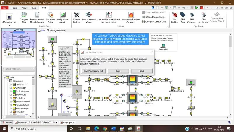
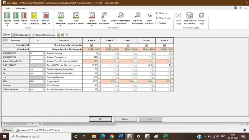
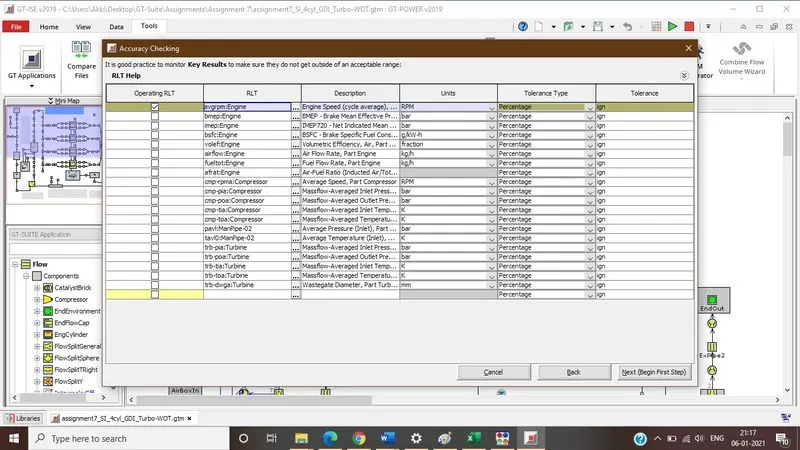
After running the simulation, the accuracy checking dialog box opens. In the "Accuracy Checking" dialog, select key RLTs to track the accuracy of the model as the conversion progresses.
Step 1: Exhaust Manifold
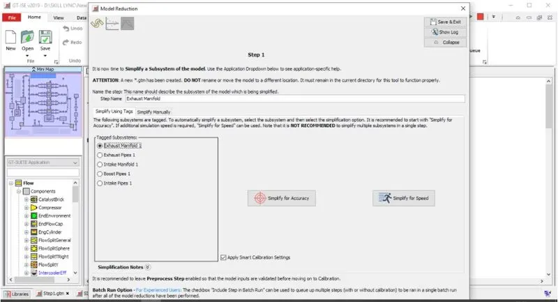
The FRM Converter should now be at the Model Reduction page, as shown below. It is now time to start simplifying the first subsystem of the model. It is most efficient to start by simplifying the subsystem that is currently restricting the time step. For high-fidelity models, this is almost always the exhaust manifold where the highest gas velocities occur, which in turn restricts the time step.
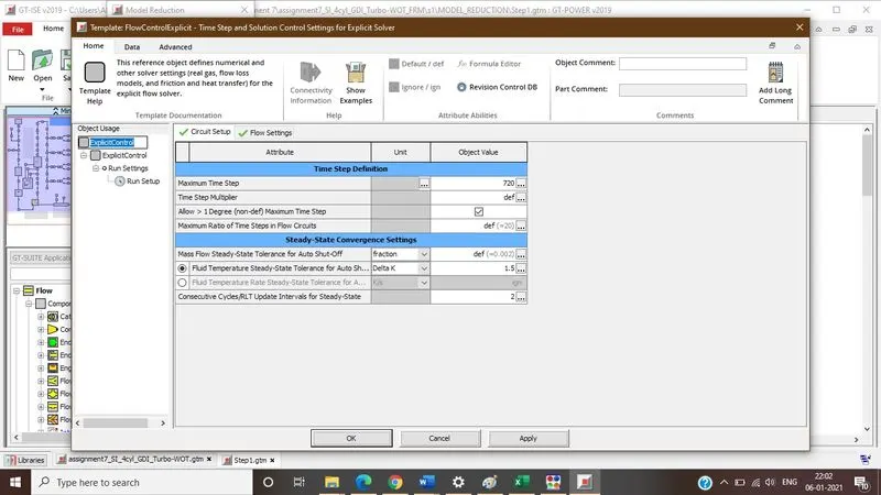
Before we apply simplifications to the exhaust manifold, the Maximum Time Step limit of 1 crank angle degree will be removed. This is a default limit that is imposed when an EngCylinder component is in the model. If the Courant Condition allows for a larger time step (by monitoring gas velocity and sub volume length in all flow components), removing this limit will allow the time step to increase in size.
If accuracy is of higher importance than run-time, choose the "Simplify for Accuracy" option. This will combine the Exhaust Ports/Runners together, and left separate from the manifold volumes. If a real-time capable model is required choose "Simplify for Speed". In this case the Ports, Runners, and Manifold volumes will be combined together at once. Moving with Simplify for Accuracy" option.
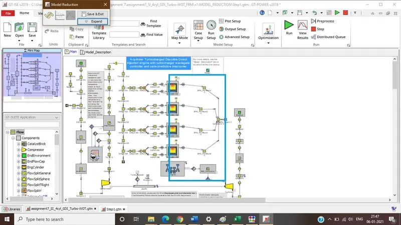
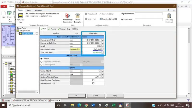
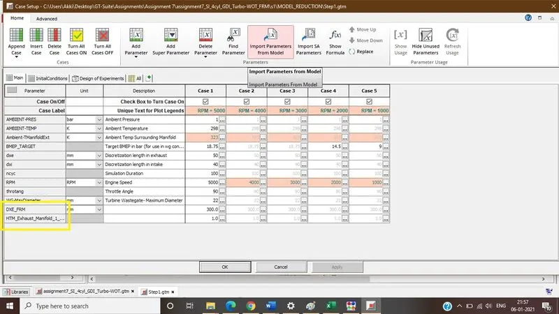
The Discretization Length in the pipe parts will be overwritten with an automatically created parameter called [dxe_FRM]. Its value will be set to 365mm.
Port Heat Transfer dominates vs. Runner Heat Transfer, therefore a parameter for the heat transfer multiplier called [HTM_Exhaust_Manifold_1_Step_1] will be automatically created in all port/runner pipes Thermal tab. This parameter will be used to calibrate heat transfer in the combined volume to assure the Turbine Inlet Temperature is maintained.
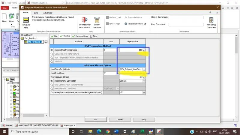
To check the created parameters
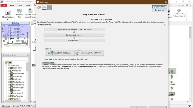
Click "Next (Calibration)"
Special Considerations for Studying Coolant Heat Rejection: If Coolant Heat Rejection must be maintained (for example, if this FRM is to be coupled with a cooling system model), then the individual Valves and Port Pipes need to remain in the model. In this case, the user would simply set the discretization length of the port pipes to [DXE_FRM] and combine the Runners and other manifold volumes into a single FlowSplit using the Combine Flow Volumes wizard (Simplify Manually tab). For the Ports, the Heat Transfer Multiplier would be used to calibrate coolant heat rejection, while the remaining FlowSplit would use a unique and separate Heat Transfer Multiplier parameter to further calibrate the Turbine Inlet Temperature. Note that leaving the original port pipes, even with the increased discretization length, may result in a significant time step restriction due to how short port pipes generally are. Therefore, their length could be artificially increased (and that additional volume taken away from the downstream flowsplit) in order to allow for a significantly larger time step. Even with the increased length (and thus increased surface area), the Heat Transfer Multiplier will still be calibrated to match coolant heat rejection.
Select Case(s) for Calibration / Open Case Setup
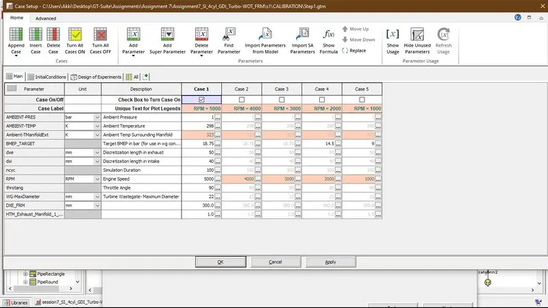
Configure Calibration - optimizing mass flow avg. inlet temp. of Turbine
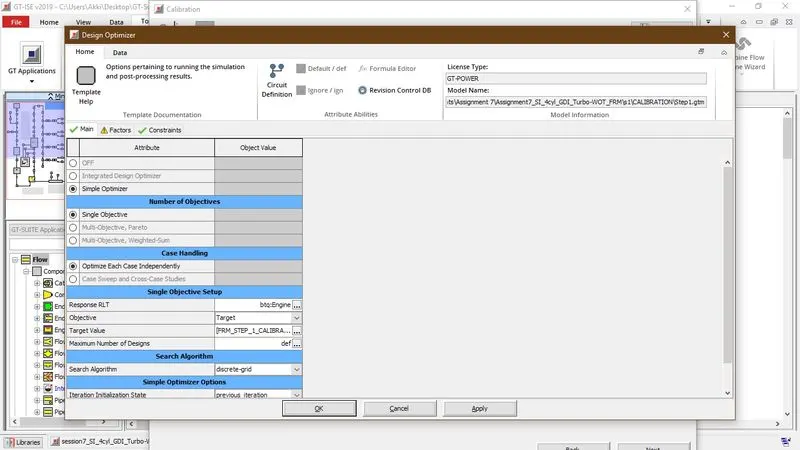
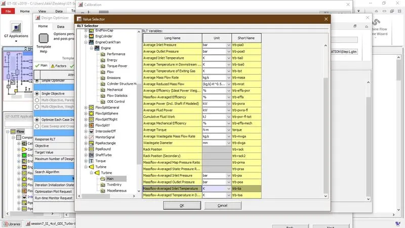
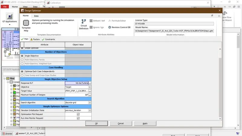
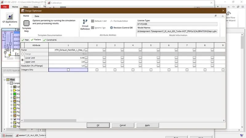
Run calibration, Once the optimization run is completed, close the simulation window and then click "Next" to go to the Results page. Note that the optimized parameter value has been automatically placed back in the model, and all of the original cases turned back On.
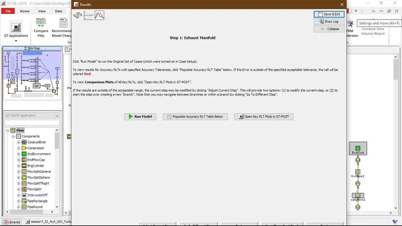
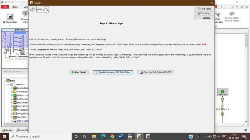
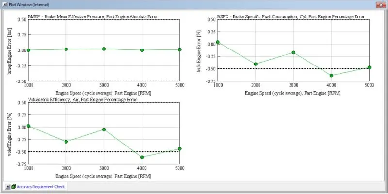
Run Model from above page Populate Accuracy RLT Table Below" to see a comparison of results for the RLTs which includes specified tolerances. If any tolerance is outside of the specified range, the tab will show a "!" indicator, and the text of the cell which contains an error outside of the specified tolerance will show up as red.
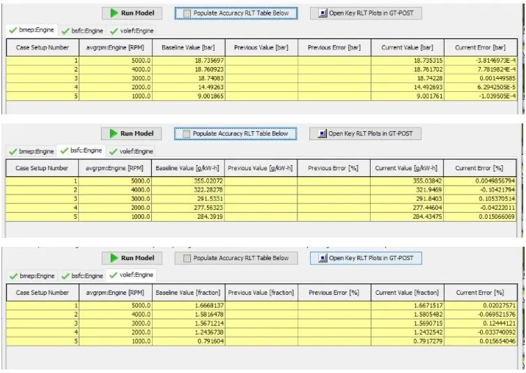
Step 1 Result
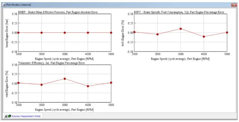
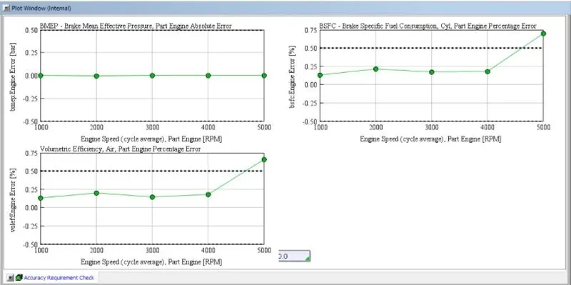
Almost zero errors are there in engine performance values after performing step 1 as compare to original model.
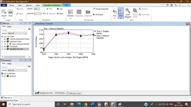
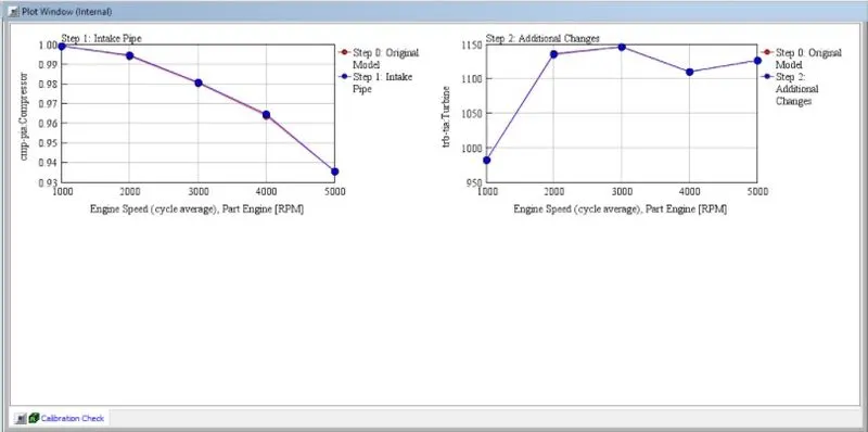
after performing step 1 turbine works almost with same speed for higher engine speed.
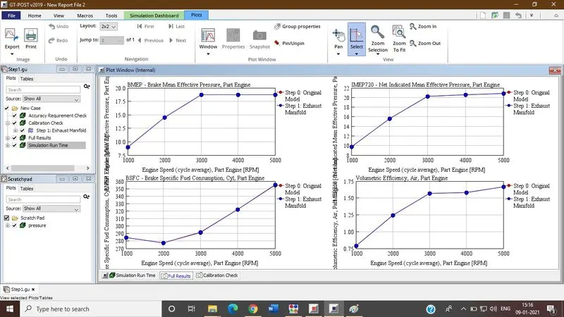
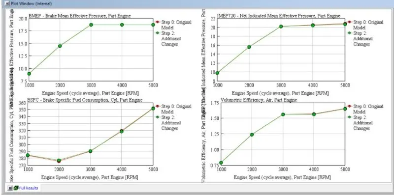
BMEP, IMEP BSFC volumetric efficiency for each engine speed is same.
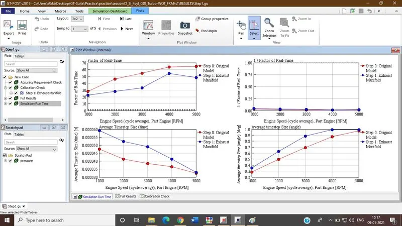
Time requires to complete the simulation for step 1 is reduced by some sec. which shows step 1 is effectively worked.
Step -2 Exhaust Pipe
For the second step of model simplification, the exhaust pipes downstream of the turbine will be simplified. Name the step "Exhaust Pipes".
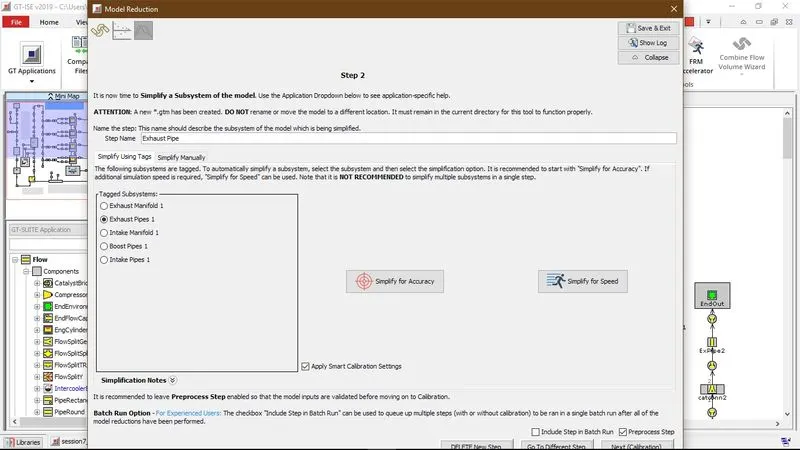
Since the pipe at the outlet of the Turbine is rather short (70mm), this pipe will be combined with the Catalyst volumes into a single FlowSplit part, see the "Simplify Manual" tab for instructions.
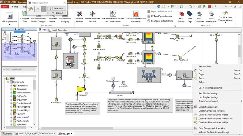
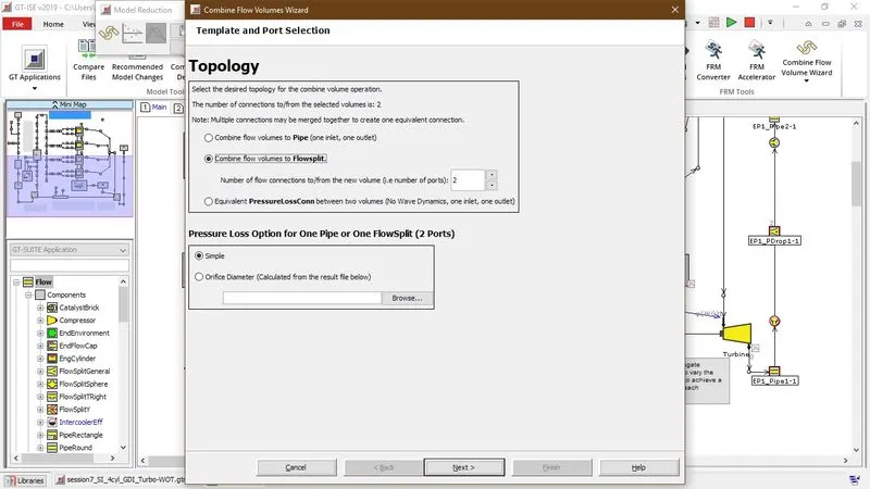
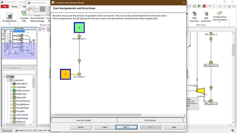
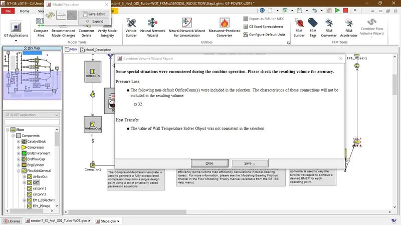
Once in the Combine Flow Volumes wizard, keep "Combine ow volumes to Flowsplit" selected and click "Next" through the wizard until the last page, "Object Attribute Definition and Object Naming". Select "EP1_PDrop1-1" at the top of the dialog, then set the object name to "CAT". The Thermal tab shows that inputs are missing. We are dealing with it later, click "Finish". Hit Close in the "Combine Volume Wizard Report".
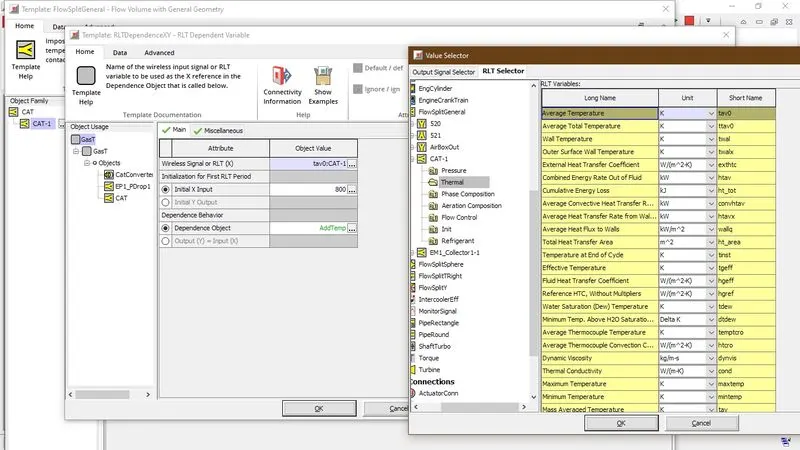
Open Case Setup and set the value of [DIA_Exhaust_Pipes_1_Step_2] to 40 mm. This is only an initial guess, and will be used to calibrate the Turbine Outlet Pressure.
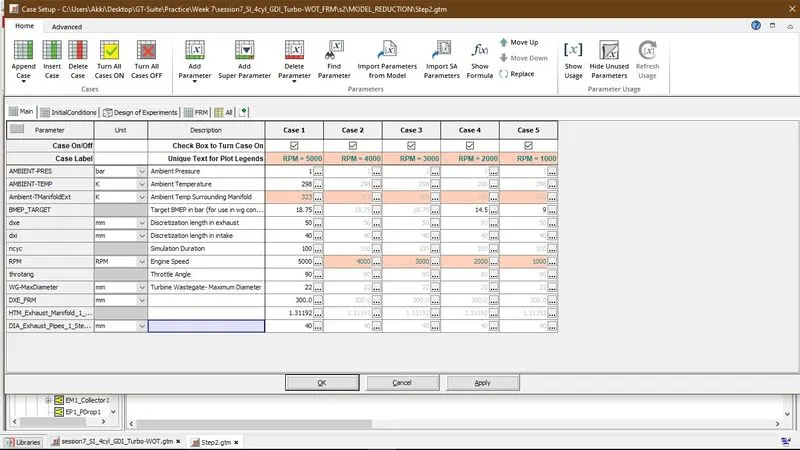
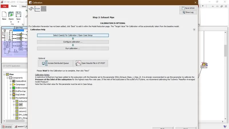
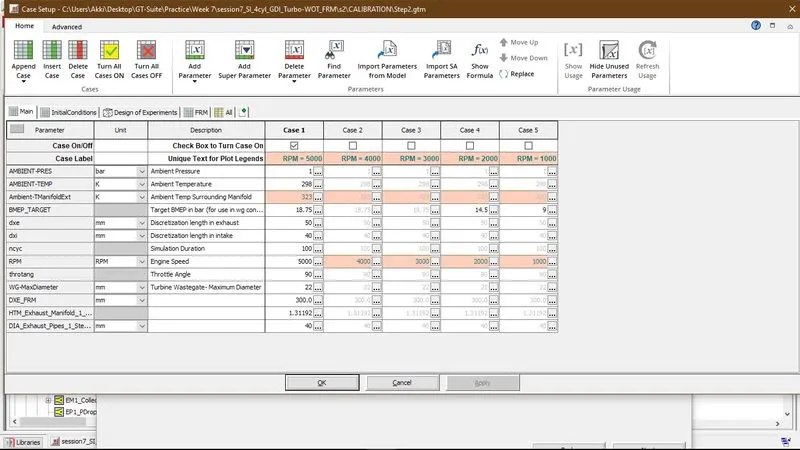
Configure calibration- optimizing mass ow avg. outlet pressure of Turbine.
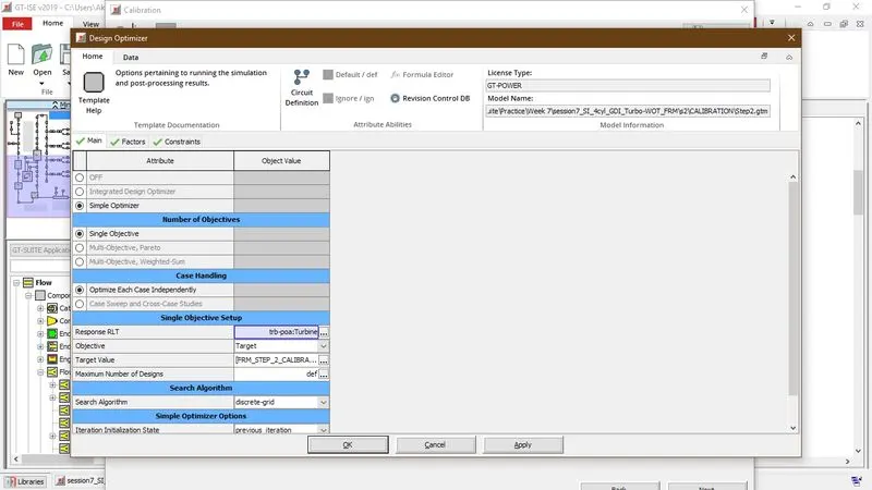
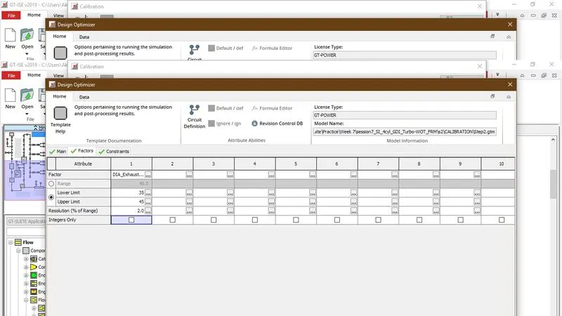
Run the calibration, and once it is finished, click "Next". In the Results page, click "Run Model" to rerun the full set of Cases. After checking model results and assuring that they are satisfactory, click "Next (Begin Next Step)".
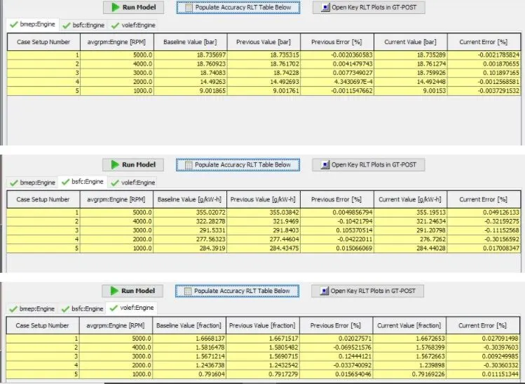
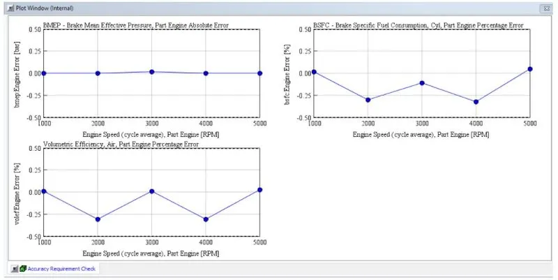
Almost zero errors are there in engine performance values after performing step 1 as compare to original model.
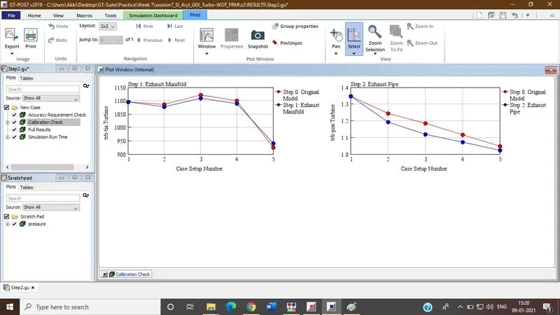
Variation occur in turbine outlet pressure is shown in above graph after performing step 2.
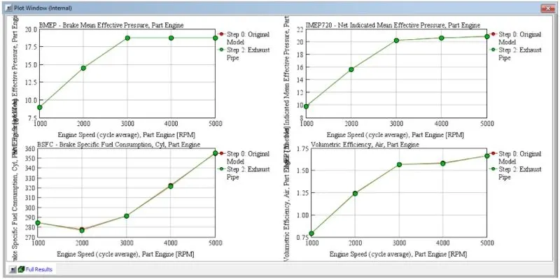
BMEP , IMEP BSFC volumetric efficiency for each engine speed is same.
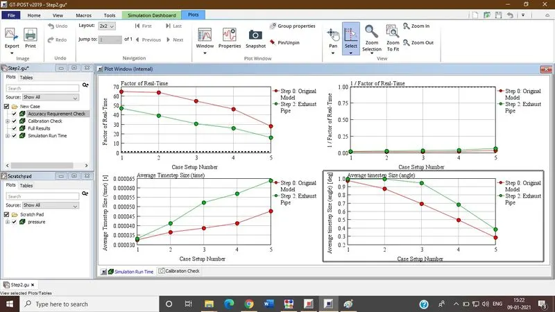
Time requires to complete the simulation for step 2 is reduced by some sec. which shows step 1 is effectively worked.
Step 3: Intake Manifold
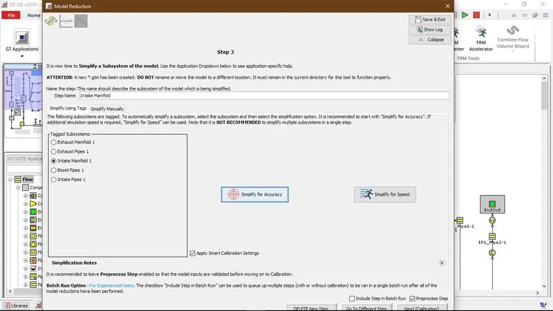
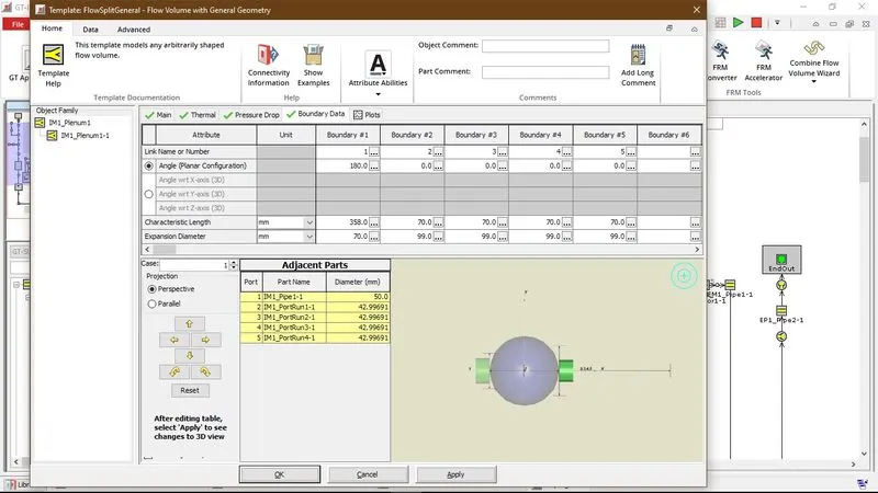
Minor modifications need to be made to the Characteristic Length and Expansion Diameter attribute values for the combined volume. The characteristic length is defined as the distance that the flow entering the boundary will travel before crossing another boundary or impacting a surface. Boundary represents the boundary between the flowsplit and IM1_Pipe1-1. The fluid entering the flowsplit in this direction can travel all the way across the plenum before impacting a surface, so the characteristic length is equal to the length of the plenum. The other boundaries are adjacent to the runners, where backflow from the cylinder would travel across the diameter of the plenum before impacting the plenum wall, which is why they are given a characteristic length of 70mm.
The expansion diameter denes the maximum diameter that the ow may expand to after entering a boundary (or contract from when leaving a boundary). For Boundary #1, it is simply the diameter of the plenum because the fluid expands from IM1_Pipe1-1 into the plenum in a straight direction. The expansion diameters for the other boundaries are equal to the plenum diameter multiplied by 1.4. This is because as the fluid backflows into the plenum, it encounters a wider cross section than the plenum diameter to expand into. For more information on Characteristic Length and Expansion Diameter.
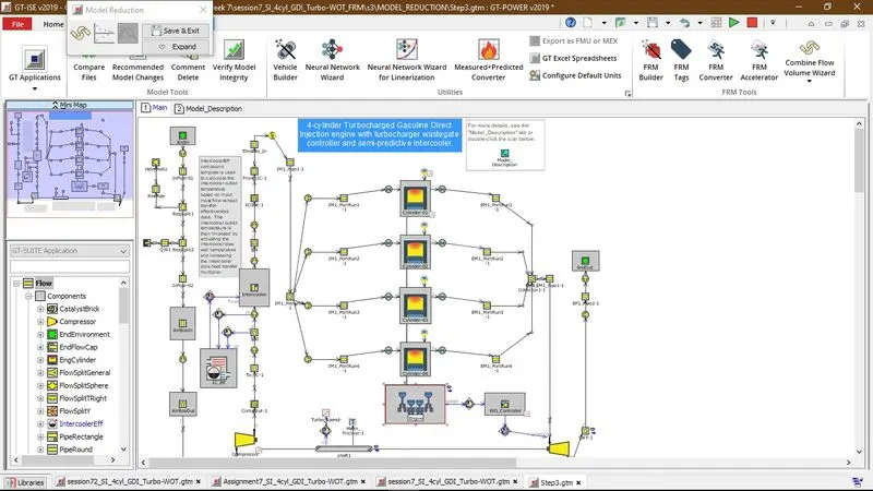
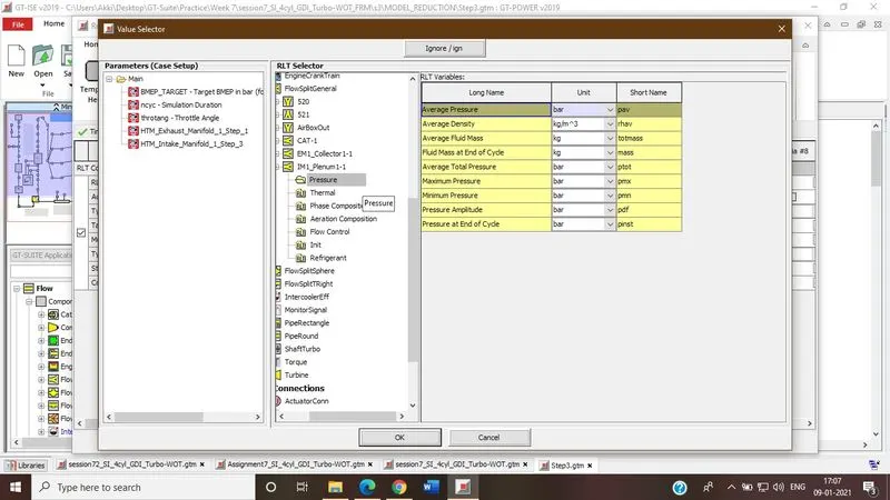
To resolve the Delete Part issue.
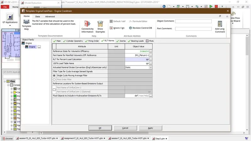
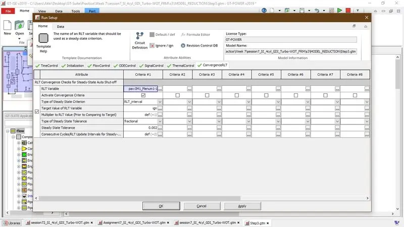
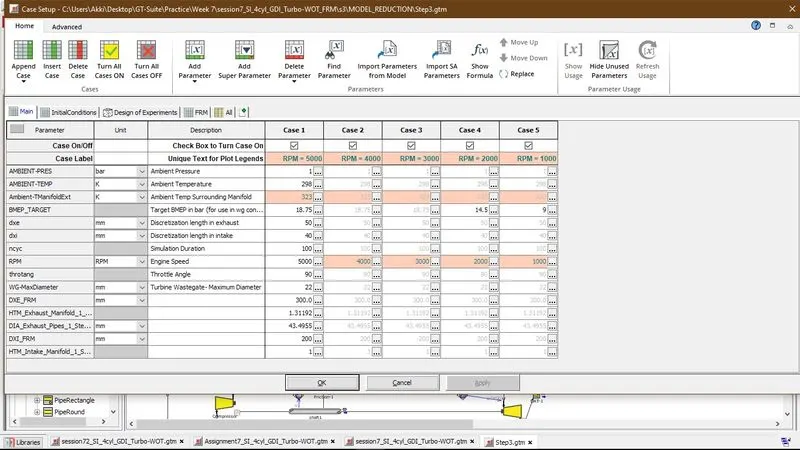
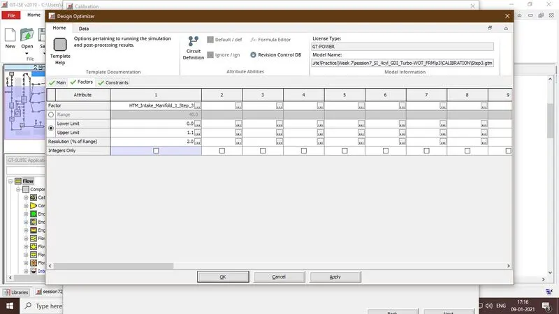
Finally, open Case Setup and check [DXI_FRM] is 200 mm, and [HTM_Intake_Manifold_1_Step_3] is 1 (this is an initial guess and will be calibrated).
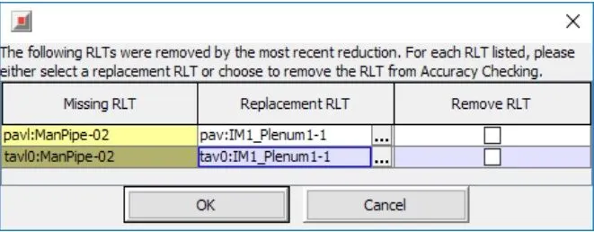
Special Considerations for Studying Coolant Heat Rejection: Similar to the Exhaust manifold, if Coolant Heat Rejection must be maintained (for example, if this FRM is to be coupled with a cooling system model), then the individual Valves and Port Pipes need to remain in the model.
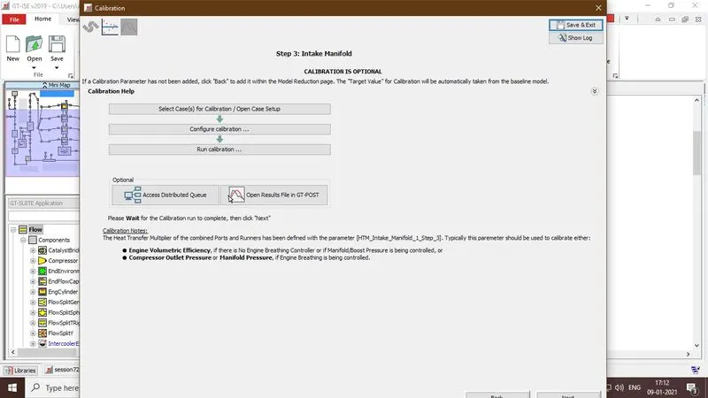
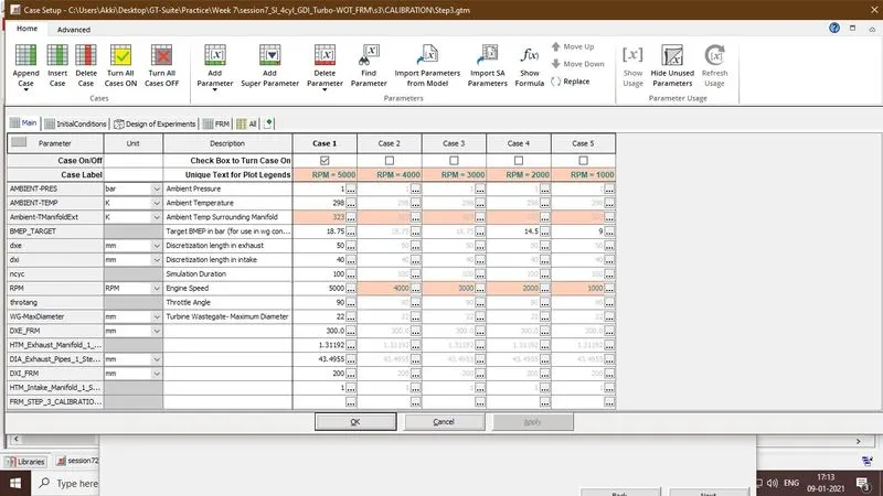
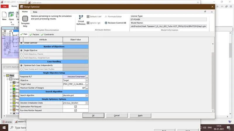
Since the wastegate controller is maintaining engine BMEP, engine air ow is also effectively maintained since the Air-to-Fuel ratio is fixed. Therefore, as the Heat Transfer Multiplier of the intake ports/runners’ changes, the resulting compressor outlet pressure will change so that engine air ow is maintained (via the wastegate controller). Therefore, the Heat Transfer Multiplier will be adjusted in order to maintain compressor outlet pressure.
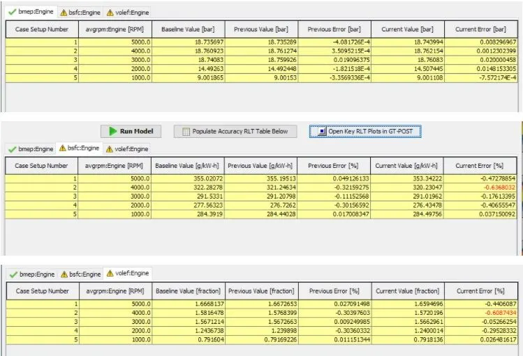
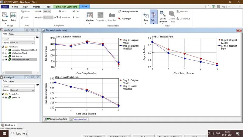
Changes in a compressor avg. mass flow outlet pressure is shown in graph no 3 due to combining intake manifold.
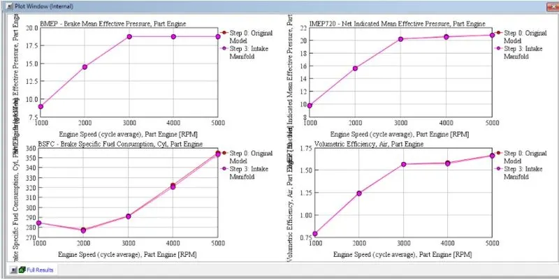
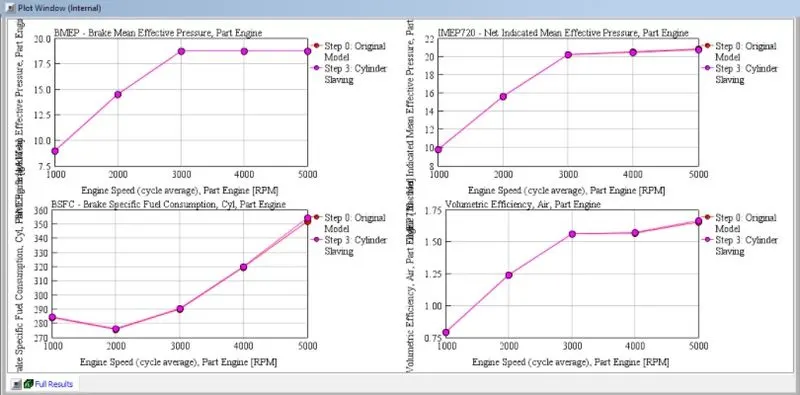
BMEP , IMEP BSFC volumetric eciency for each engine speed is same.
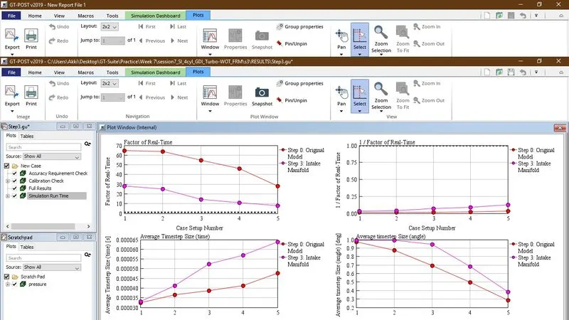
Time requires to complete the simulation for step 3 is reduced by some sec. which shows step 1 is effectively worked.
Step 4: Compressor Outlet Pipes
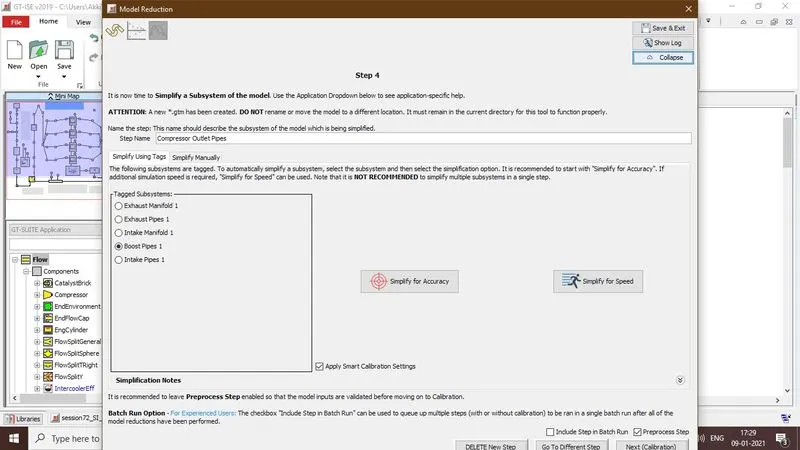
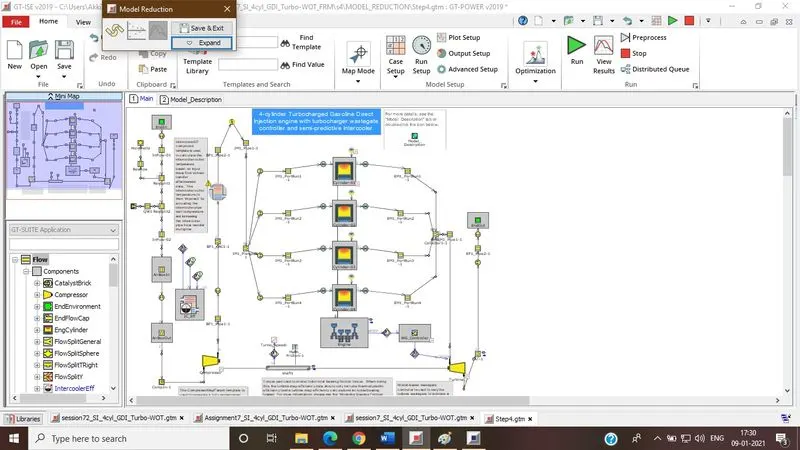
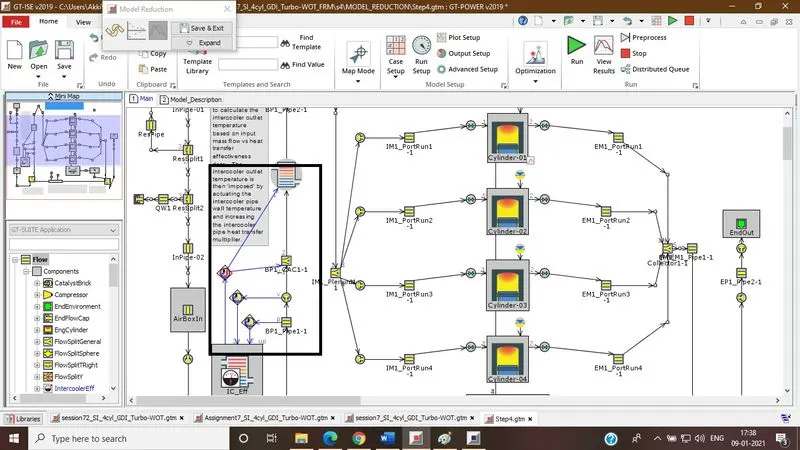
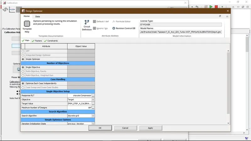
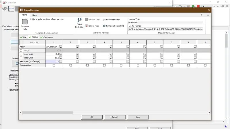
Name the step "Compressor Outlet Pipes". Select Boost Pipes 1 from the Tagged Subsystems list. Click on "Simplify for Accuracy". Collapse the FRM Converter to provide space to work in the model map. Since the intercooler core (previously a bundle of pipes) has been replaced with a FlowSplit and "HeatExchangerConn" part. The "BP1_CAC1-2 HeatExchangerConn" part will be used to assure the intercooler outlet temperature is maintained. Double-click on the "BP1_CAC1-2 HeatExchangerConn" part and set the Imposed Fluid Temperature to 300 (this will be overridden), then click OK. Open the "BP1_CAC1-1" Flowsplit part, go to the Thermal tab and select Imposed Wall Temperature. Set the temperature to 300 (this will be overridden), then click OK. Finally, reconnect the Control links, sensing Upstream Temperature from "BP1_Pipe1-1" Pipe and Upstream Mass Flow Rate from the "6” OriceConn upstream of the "BP1_CAC1-1" Flowsplit, and sending the actuator output to both "BP1_CAC1-1" Flowsplit (actuating Wall Temperature) and to the HeatExchangerConn (actuating Imposed Fluid Temperature).
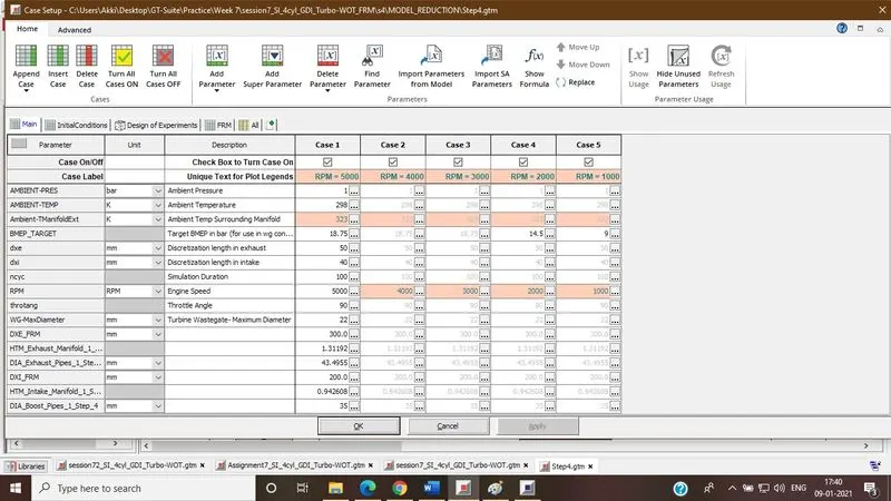
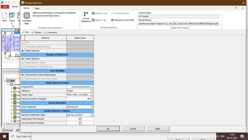
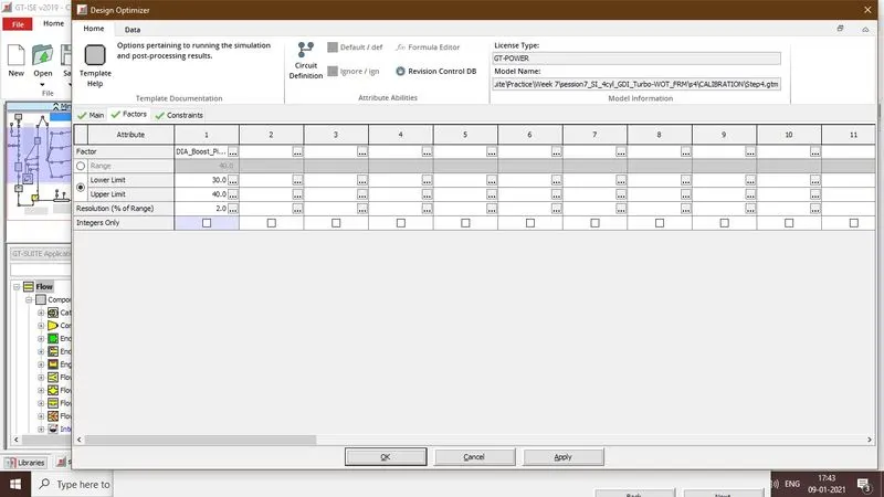
Since the wastegate controller is maintaining engine BMEP, engine air ow is also effectively maintained since the Air-to-Fuel ratio is fixed. Therefore, as the effective diameter of the Intercooler changes, the resulting compressor outlet pressure will change so that engine air ow is maintained (via the wastegate controller). Therefore, the Intercooler Diameter will be adjusted in order to maintain compressor outlet pressure.
- Intake Pipes
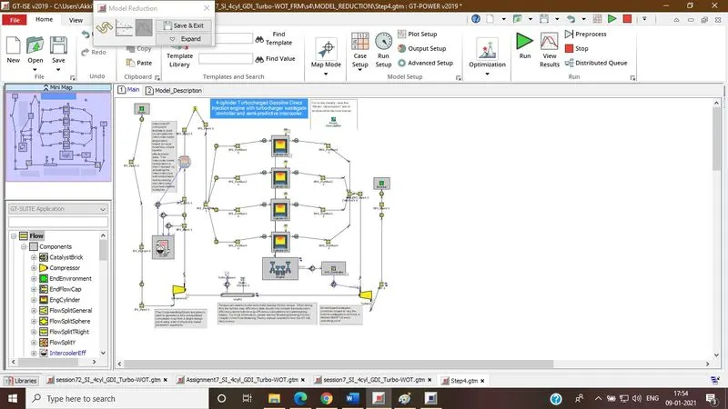
Name the step "Intake Pipes". Select Intake Pipes 1 from the Tagged Subsystems list. Click on "Simplify for Accuracy". Collapse the FRM Converter to provide space to work in the model map.
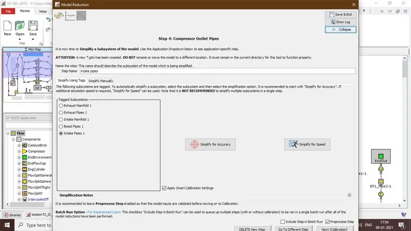
Go into Case Setup and set the value of [DIA_Intake_Pipes_1_Step_5] to 45 mm (this is just an initial guess)
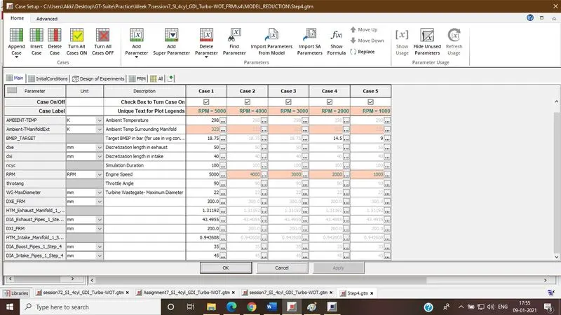
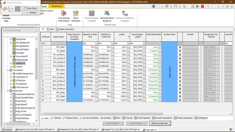
Since every subsystem has now been simplified, we will assure that there are no remaining pipes with short discretization lengths.
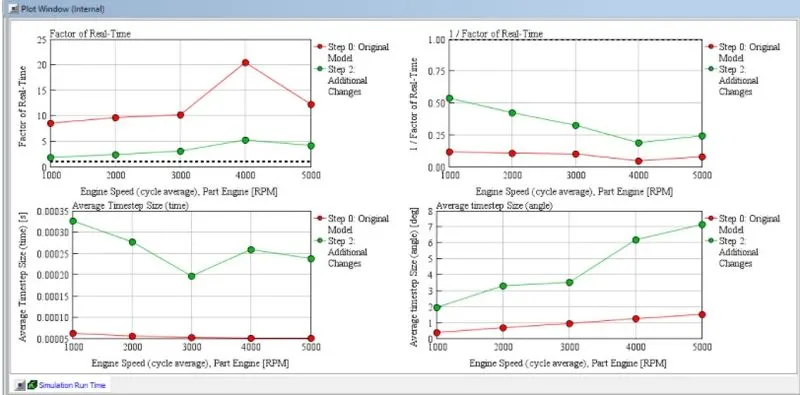
At this point, we should have a Fast-Running Engine Model running at a Factor of Real-Time of around 5 xRT and with very high accuracy.
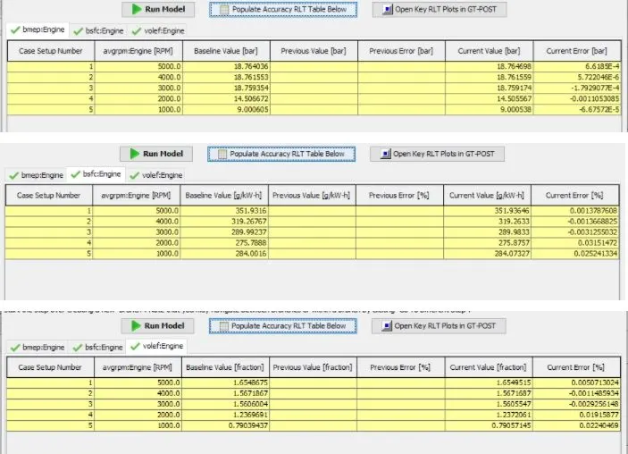
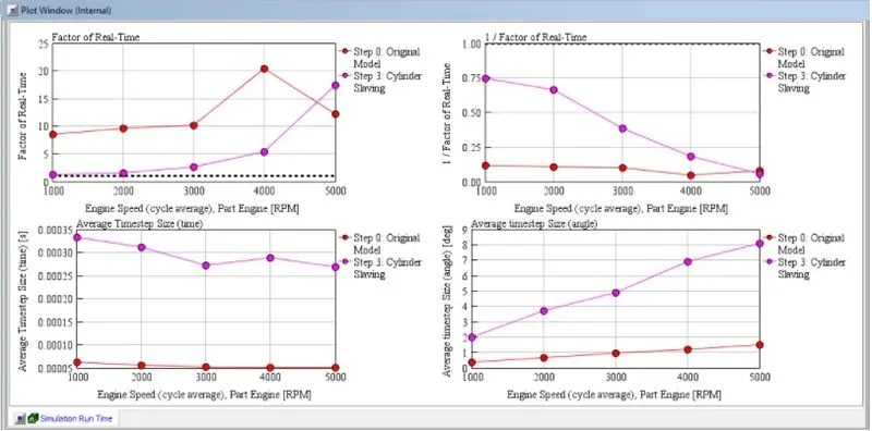
At this point, we should have a Fast-Running Engine Model running at a Factor of Real-Time of around 5 xRT and with very high accuracy. The Simulation Run Time can be checked clicking on the "Open Key RLT Plots in GT-POST" and plotting the Simulation Run Time data. The RT factor can be accessed as well by opening the model result file -> Case RLT tab -> Global -> Special -> "Factor of Real-Time".
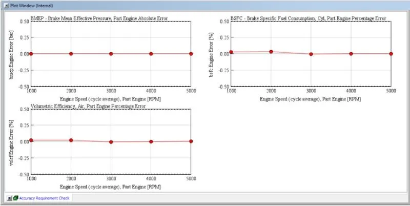
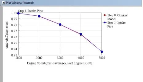
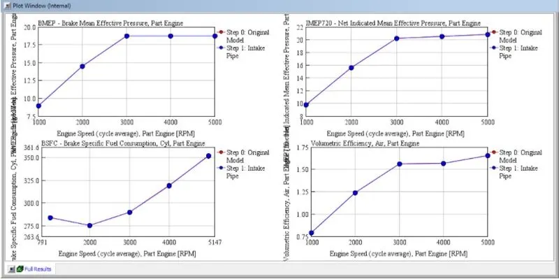
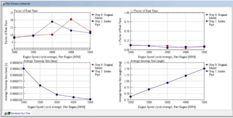
At Step 5-time step size is almost zero.
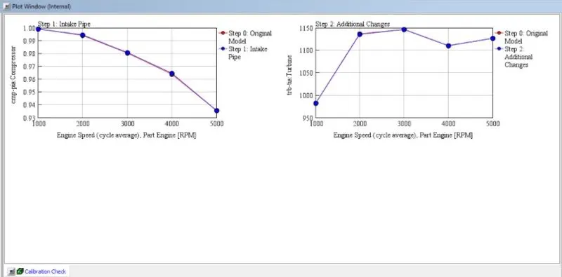
Step 6: Additional Changes
Name the step "Additional Changes". Select Exhaust Manifold 1 from the Tagged Subsystems list. Click on "Simplify for Speed".
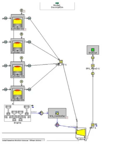
Click "Next (Calibration)" to pre-process the model and continue to Calibration. In the Calibration page, leave all cases enabled for calibration. This may take some additional time to calibrate vs. only calibrating for Case 1, but it will result in better accuracy across all operating conditions. Under "Configure calibration…", change the Response RLT to the Turbine Massflow-Averaged Inlet Temperature (trb-tia:Turbine). Set the lower and upper values for HTM_Exhaust_Manifold_1_Step_6 of the range at 0 and 2, respectively. Set the Resolution (% of Range) to 1.
Run the calibration, and once it is finished, click "Next". In the Results page, click "Run Model" to rerun the full set of Cases. Check the model results and assure that they are satisfactory. The model should now be running around 1 xRT. In the FRM Converter, click "Next (Begin Next Step)".
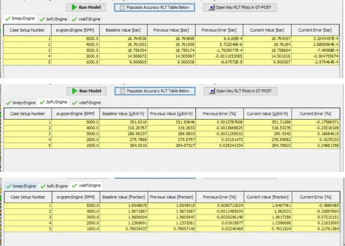
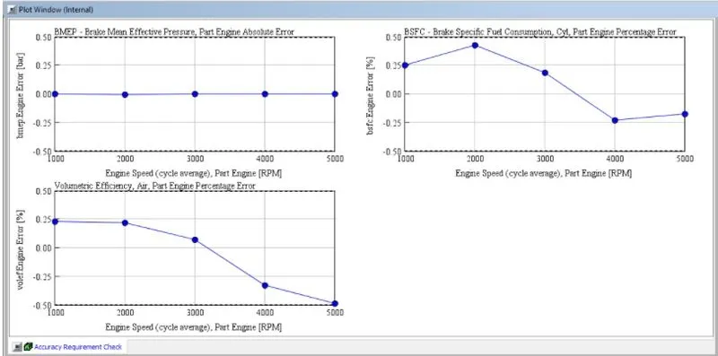
Step 7: Cylinder Slaving
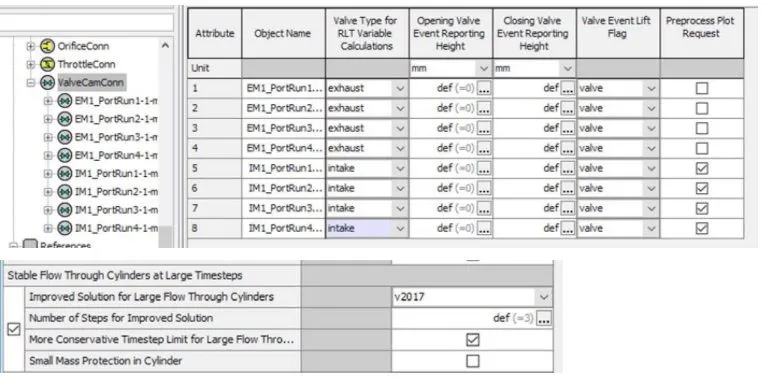
For the full cylinder slaving to function, each Valve must be specified as either an Intake or Exhaust valve. Find the ValveCamConn template in the model tree on the left and select "Edit Parts in Spreadsheet" view. The intake and exhaust valves are easy to distinguish. The intake ones start with "IM1_PortRun” and the exhaust ones start with "EM1_PostRun". Go to the Output folder and set "Valve Type for RLT Variable Calculations" to "intake", respectively "exhaust “Expand the FRM Converter and click "Next (Calibration)" to pre-process the model and continue to Calibration. Calibration will not be performed for this step, so simply click Next to get to the Results page without performing calibration, then click "Run Model" to run the full operating range with this latest modification.
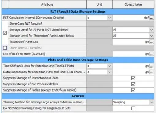
With the final run complete, view the results and assure that the accuracy is acceptable. The runtime of the model should now be below 1 xRT for all operating conditions. Note that the runtime is affected by the CPU, stored data, monitors as well as any other processes that are running while the simulation is progressing, so it is possible this final model may not run below 1 xRT on a given machine. To achieve faster runtime, suppress storage in Output Setup -> Data Storage like Instantaneous Plots, Time RLTs and if run local turn off monitors. Step 8: Real-Time Solver (optional)
Click "Next (Begin Next Step)" in the FRM Converter. Name this new step "Real-Time Solver", then collapse the FRM Converter. To run with the real-time solver, the license type of the model must be changed. However, certain templates are not allowed with the real-time solver, and so they must first be removed from the model.
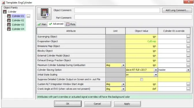
In the Main assembly delete the Turbo_Speed-2 monitor part coming off of the turbocharger shaft. Next, right-click on one of the EngCylinder parts and choose "Edit Parent Object". Go to the Advanced folder and set "Evaporation Object" to "ign" and click OK. Next, open the WG_Controller, go to the Convergence folder, and set "Steady State Error Tolerance" to "ign" Lastly in the GT ISE toolbar go to the Data tab and click the arrow next to "Delete Unused Objects" and choose and set Steady State Error Tolerance to ign . Lastly, in the GT-ISE toolbar, go to the Data tab and click the arrow next to Delete Unused Objects and choose "Objects and Templates". Expand the FRM Converter and click "Next (Calibration)" to pre-process the model and continue to Calibration. Calibration will not be performed for this step, so simply click Next to get to the Results page without performing calibration, then click "Run Model" to run the full operating range with the Real-Time Solver.
Note that most RLTs are ignored when running the RT solver in order to improve the simulation speed. Therefore, certain results will not be automatically compared using the "Populate Accuracy RLT Table Below" or "Open Key RLT Plots in GT-POST" buttons. However, they can still be used for certain results that are stored (e.g., Engine BMEP and ow component Temperatures and Pressures).
To complete the FRM Conversion process, click "Finish" in the FRM Converter. This will save the final model into the SI_4cyl_GDI_Turbo-WOT_FRM_FINAL subdirectory. To continue working on the model, or to review the process, the *.frm le can be reloaded at any time into the FRM Converter to continue the process where it was left off.
Step 8: Real-Time Solver (optional)
Running an FRM with the Real-Time Solver (optional, only available with an RT license
FRM Builder Approach
This is another way of creating FRM model right from beginning. No detailed model is used in it. It gives us various options to build desired specification engine.
Build FRM Model for following configuration using FRM builder approach
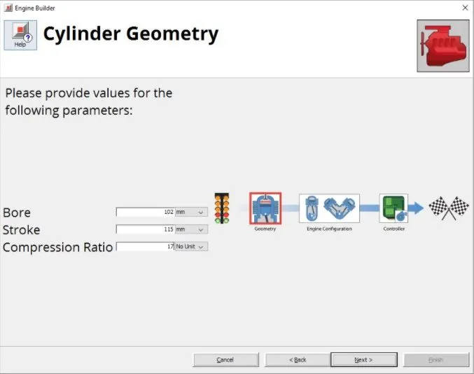
Bore 102 mm
stroke 115 mm
CR 17
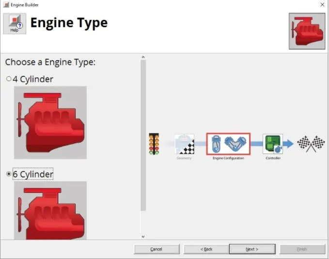
No of cylinder 6
CI engine
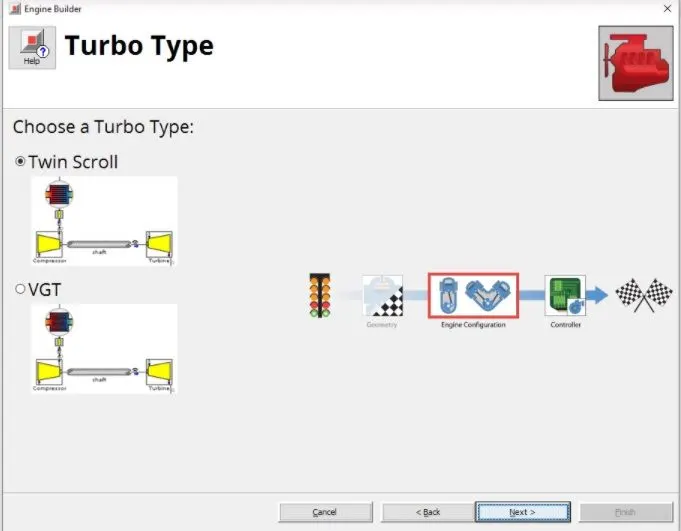
Twin Scroll Turbine
GT Controller Procedure
Procedure
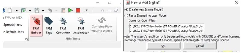
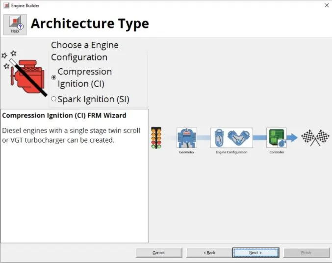
Choosing Engine type
Setting the cylinder dimension
Selecting Turbocharger type
Selecting number of engine cylinder
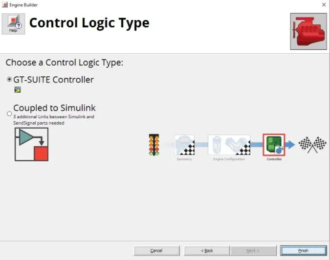
FRM Built model
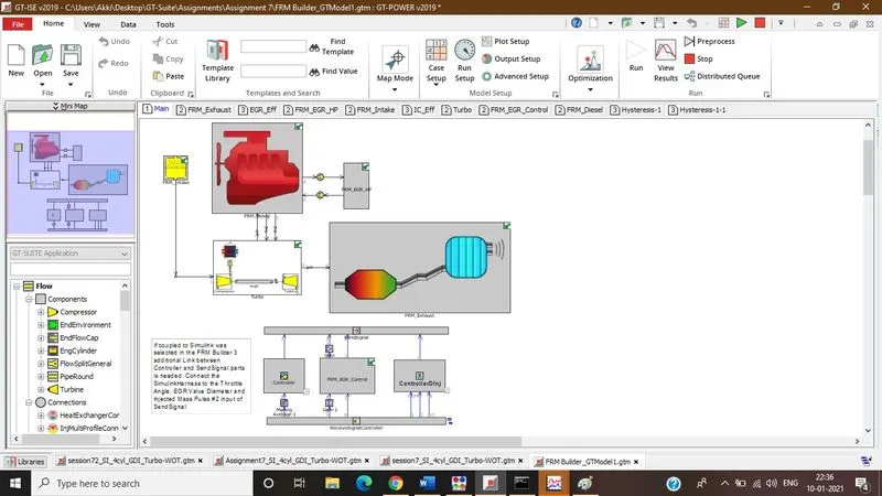
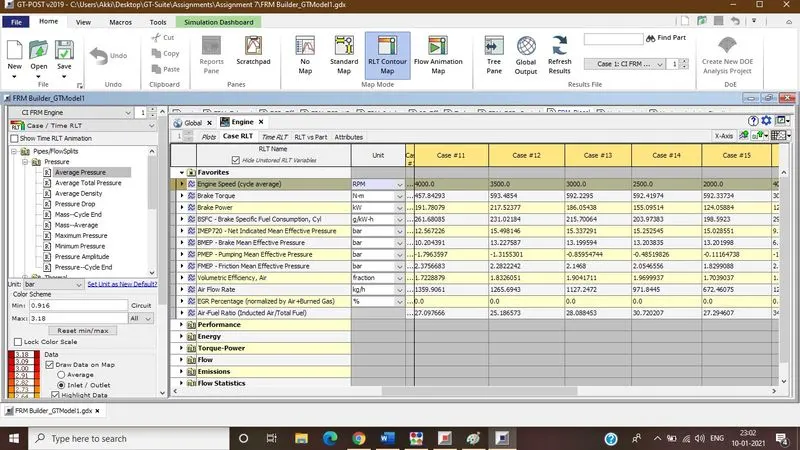
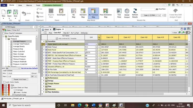
The above model is run with the 25 different cases which are formed out of varying five operating parameters. Engine is operated within the range of 4000 to 2000 rpm with varying BMEP and Boost pressure. Engine is simulated for 100% load condition to 20% load Conditions.
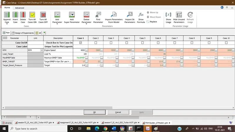
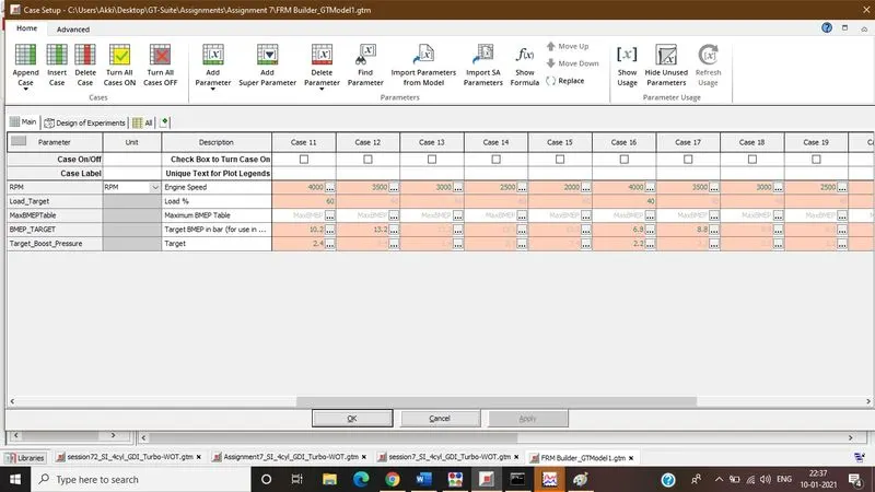
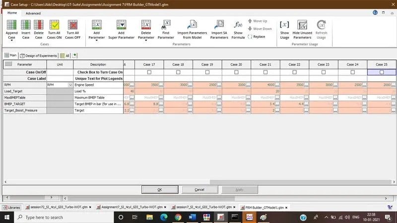
All of the 25 cases run around 7 min which shows the machine run time required for the FRM model is much less than detailed model of engine.
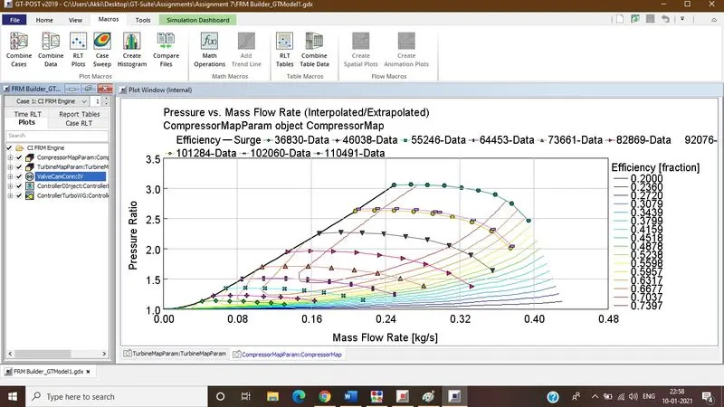
compressor efficiency reaches towards 0.73
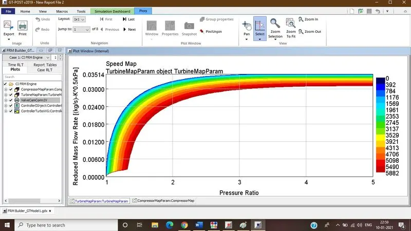
Turbine efficiency reaches towards 0.74 when operated on high engine speed and high pressure ratio.
For Full (100%) load Condition
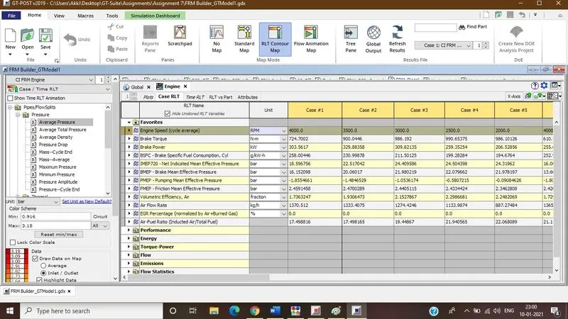
for full load condition FRM model has achieved the targeted values also A/F increases upto 22 for low engine speed.
For Full (80%) load Condition
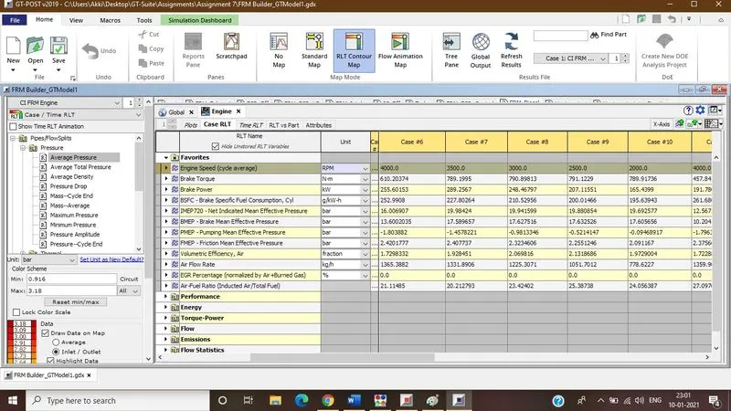
All the BMEP targets are achieved and A/f increases up to 24 for low engine speed.
For Full (60%) load Condition
For Full (40%) load Condition
For Full (20%) load Condition
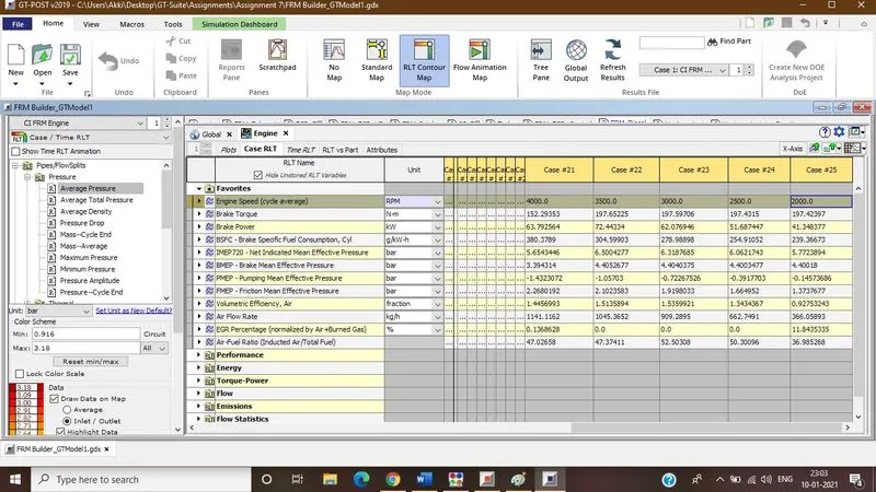
So, from the above results it can be seen that engine with 100% load requires more torque and power than part load condition that means FRM model creates results equivalent to real detail engine model with fastest simulation time.
The FRM engine can be able produce 990N-m torque at 2500rpm and it can produce 329.9Kw power at 3500 rpm at full load condition.
BSFC range of this model is 380-194g/Kwh for various rpm and load conditions.
A/F ratio range 17.45-52.5.
Inferences
FRM model help us to increase the time step size and to decrease the simulation time. These two means are often accomplished at the same time by lumping various flow volumes together which will reduce the total number of sub volumes and also allow for a larger time step size by increasing the effective sub volume length (which is responsible for the time step size). In addition to simplifying and combining flow volumes, there are additional solver options that can reduce the number of calculations per time step and, thus, further decrease the run time without changing the time step size.
This tutorial 9 covers the process of creating a Real-Time capable Fast Running Engine Model from a detailed, high-fidelity engine model. While this tutorial 9 shows a specific set of steps, note that each engine model is unique and so the steps required to convert a detailed model will depend on the complexity of the model, as well as on the goals of the end user. For certain applications, such as Vehicle Thermal Management where engine coolant heat rejection must be maintained, the procedure may differ slightly in order to maintain certain key results. While this FRM process will focus on preserving general engine performance results, special considerations will be noted along the way.