Challenge

Frontal Crash Simulation

YYash Ghate16 Jun 2022

OBJECTIVE: To run the simulation for frontal crash after fulfilling the requirement given below and plot energies and forces in Hypergraph 2D to make sense of the animation.

ABSTRACT: Crashworthiness is a term that refers to the quality of the response of the structure when it is subjected to the impact loads. In layman’s terms, it is the ability of the structure to protect its occupants during an impact. As the focus of consumers has also shifted towards the safety rating of the cars, the automakers are compelled to go through a mandatory crash test. However, this crash testing is not a one-time business. If a car does not perform well in this test, it is given a lower rating. So, the company cannot pitch the car as safe care while marketing. Thus, the manufacturer makes some changes in the design, makes a prototype, and again sends it for testing. If the car does not perform well again, the process continues. This entire process takes a lot of money. Hence, FEA is a cost-effective method that provides similar results and saves a lot of money. In this project, I have run the simulation of a car model for a frontal crash. As the project was done on the student version and looking at the performance of the system that I am working on, only critical components that play a role in the frontal crash are taken into account.

REQUIREMENTS:

Check unit system and either follow[Mg mm s] or [Kg mm ms]
Create an Appropriate interface with recommended parameters and friction 2
Make sure there are no penetrations or intersections
Correct rigid body issues if any
Crete rigid wall with friction 0.1
Add mass to reach the target of 700Kg
The initial velocity of 35mph
Time step: 0.5-0.1 ms
Run time: 80ms
Use a model checker to ensure good quality

Output Request:

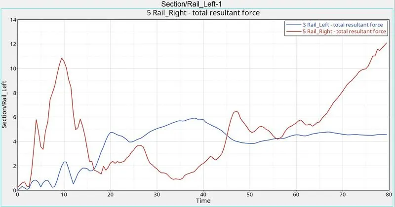
Sectional Force in the rails at node id 174247
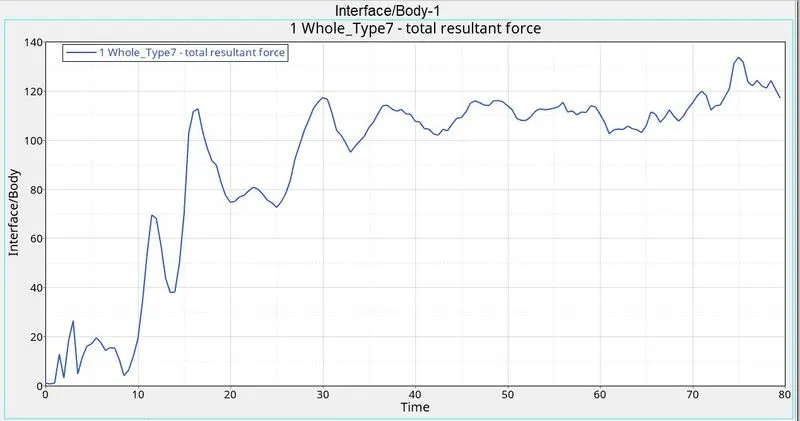
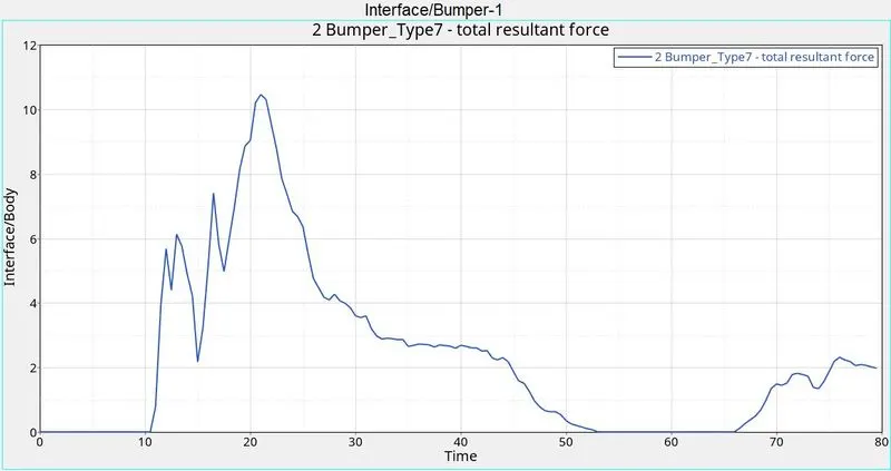
The axial force received on the rails from bumper
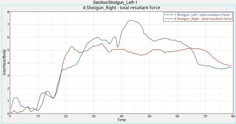
Shotgun cross-sectional forces
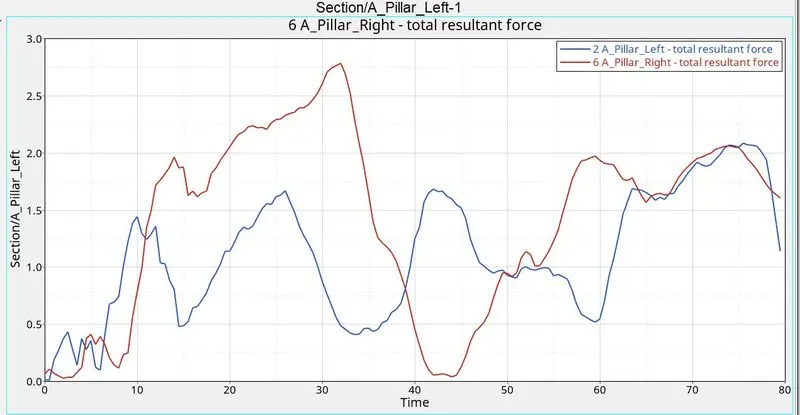
A pillar cross-section
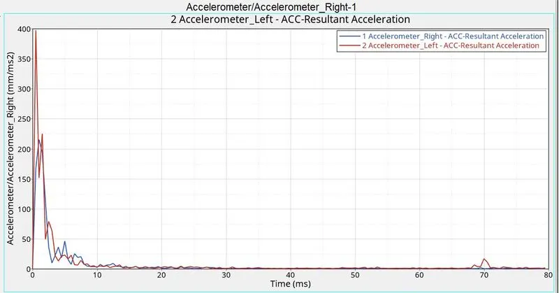
Acceleration curve received on the accelerometer at the base of B pillar
Intrusions on the dash wall 66695 and 66244

PROCEDURE:

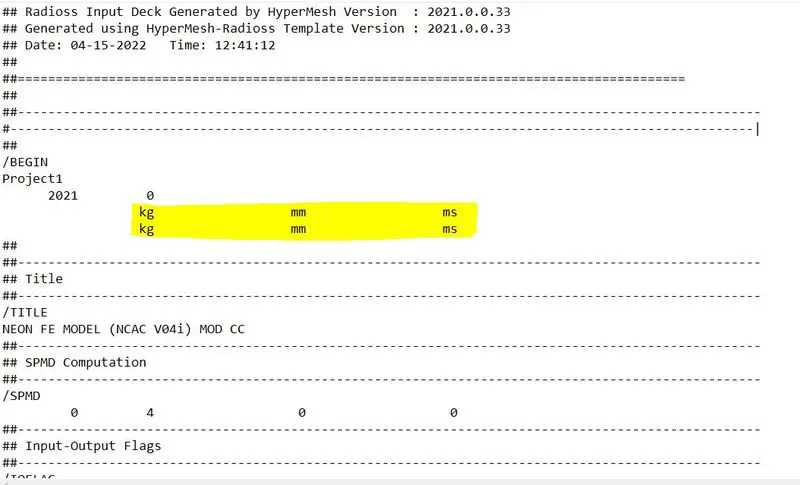
Step-1: Checking the unit system. This can be done from the software GUI or from the starter file. I prefer doing it with the latter method. Just open 0000.rad file and check the mentioned unit system. In this case, the default is Kg mm ms which is considerable. Thus, I did not make any changes to this unit.

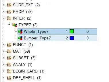
Contact interface: They are defined to model how parts interact when they come into contact with each other. We have used contact interface Type-7 which uses the penalty method for calculation.

Penalty method: It treats the behavior of slave nodes and master segment as that of the spring that generates resistive forces as a function of penetration. When the slave nodes approach the master penetrates into the gap of the latter, a 1D spring is created between them whose stiffness is auto-calculated. This stiffness will determine the time step of this contact.

Interface Parameters:

Igap: How the size of the gap is calculated
Gap(min): Minimum gap for activation of the interface
Inacti: Action it takes if initial penetration exists
Isft: Affects how the stiffness of the interface is calculated
Iform: Friction formulation
Stmin: Minimum stiffness to use in the interface
Idel: What to do with slave nodes and master segments in case of element failure

Step-2: Checking interface, creating new interfaces with recommended properties. In the model, we can see some interfaces which are really not needed for the simulation. So I followed the below process to create a new interface.

Go to solver browser and delete existing interfaces.
Right-click in the solver browser > Create > INTER> Type 7
Rename it as body as it is for the entire body to check self-impact.
Select slave nodes as all the nodes in the model and master segment as all the elements in the model
Now insert the required parameters as given below

Interface parameters recommendation:

Igap: 2 or 3
Gap(min) <= 0.5mm
Inacti: 6
Istf: 4
Stmin: 1000N/mm
Idel: 2
Iform: 2

This was to check the forces and energies on the model. We have to repeat the same process and create another type-7 interface for the bumper to study forces.

Initial penetration or intersection: This condition occurs when the slave node is present in the gap region of the master segment. This is an undesirable situation as it can cause a locking situation leading to failure as there will be initial repulsive forces in the simulation which cause the error. Hence, they should be dealt with. We can fix this problem by any of the following two methods:

Using Inacti=6 value in the contact interface definition. This is to reduce the gap and scale it so that the slave node is not in the new gap region of the master segment.
Fixing the penetrated nodes manually in Hypercrash or Hypermesh. It is basically pulling the nodes out of the gap region of the master segment.

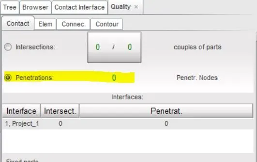
Step-3: Checking penetrations. In this project, after giving interface 7 contacts for self-impact and for studying the contact forces in the bumper, the penetrations were found to be zero. To check the penetration in the model:

Go to Tools > Penetration check
Select the invoke penetration option > select all the components and check if there are any penetrations.

In this case, there were no penetrations in the model.

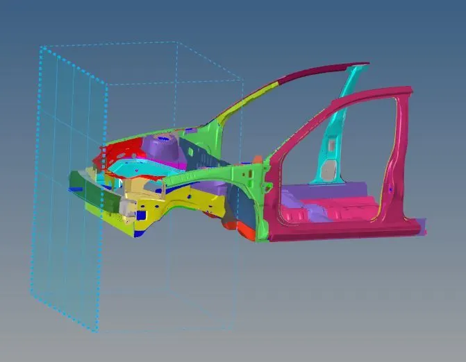
Rigid wall: As the name suggests, it will behave like a body that will not let anything pass through it. It is interesting to note that the rigid wall is just an imaginary or virtual representation.

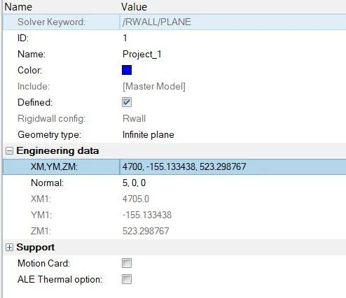
Step-4: Defining a rigid wall. I have followed the following method to create a rigid wall in the model.

Go to Solver browser > Right-click > Create > Rwall > Plane
As the wall will be at the front of the car, select a node of the bumper for reference. Then we can play around with the coordinates to place the wall in a proper position.
Make sure that there is a small gap between the car and the wall for a crash situation. If this gap is more, the solver will take more time to run the simulation. I have kept a gap of 50-100mm.
Set the normal in x-direction as -1. This will change the direction of the search tolerance.
Select sliding with friction option and keep friction value as 0.1.
Keep search tolerance value of 1150-1200. The nodes coming into this region will be considered as slaved for the master rigid wall.

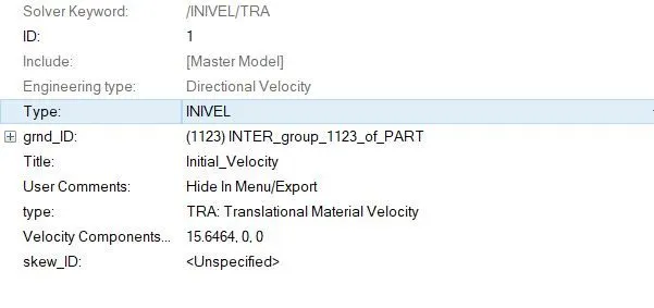
Initial velocity: This is just an initial push that we give to the model. As this velocity does not change with time, we do not have to create a function to define the velocity.

Step-5: Create initial velocity.

Go to solver browser > Right-click > create > boundary conditions > INIVEL
Select all the nodes present in the model
Give an initial velocity of 35MPH (15.6464mm/ms) in a positive x-direction

Step-6: Adding mass to the system. The mass of the given model was about 188 Kg, which is very less for a car model. This mass only made sense if we consider the model which is BIW. However, for running a simulation for the crash, we must consider a car model thus we must add mass to this model. We can add mass where other components will sit like the seat and passenger. The aim is to reach 700kg while maintaining a proper Centre of Gravity location.

Go to Solver browser > Right-click > ADMAS
Select type 1 which will distribute the given mass over the selected area
Select the nodes and keep on adding mass till the CoG reaches the desired position.

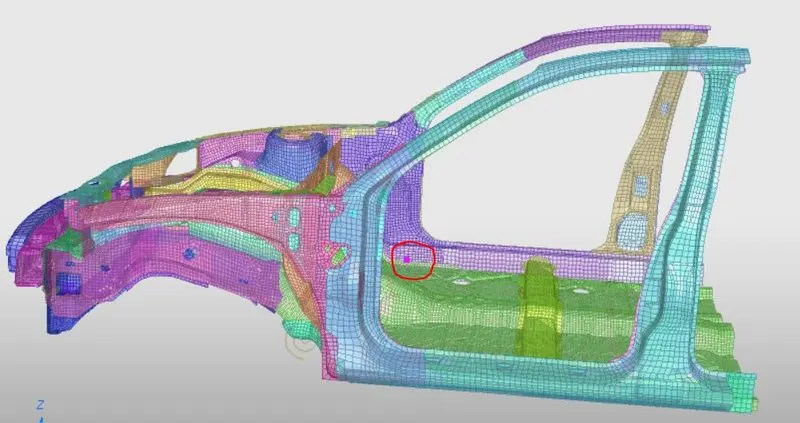
FIG. OLD CoG

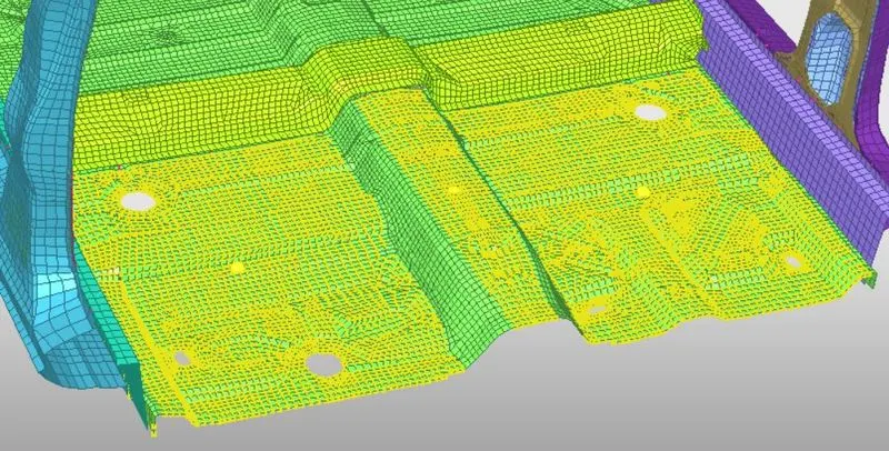
FIG. ADDED MASS

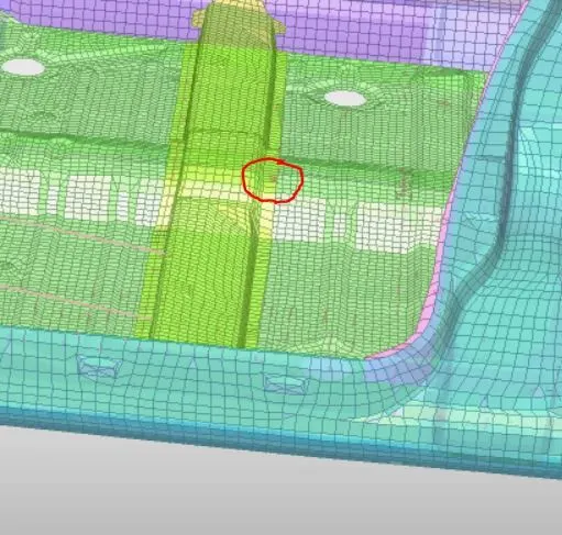
FIG. NEW CoG

Time-step: Critical time step is the time needed for the information to cross the smallest distance in an element. We can say a model is stable if the current time step (Time required for information to travel from one node to another) is less than the critical time step of the model. If the current time step falls below the critical time step, the model is not stable. In addition, if the time step is very small then the time to run the simulation will be very large. Thus, to speed up the simulation time, we introduce cards like NODA/CST that will add the mass to that node if the time step falls below the minimum time step value.

Step-7: Minimum time step value of 0.5ms. If the time step falls below this value, the solver will add mass to the node and increase the time step of the model. Basically, this is the mandate by NODA/CST card in this model.

In model browser > Cards> ENG_DT_NODA
Change the Tmin value to 0.005

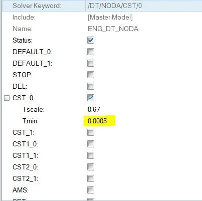
Step-8: Creating sections. Sections help us to study the forces in a particular part/section of the model. For this project, I have created 6 sections namely left and right A-Pillar, left and right rails, left and right shotguns. Creating sections follows the same procedure.

Go to Solver browser> Right-click > Create a Frame> MOV
Define origin point, x-axis and xy-plane
Go to Solver browser> Right click> SECT> SECT
Select an N1, N2, and N3. Select frame the one which we created.
Right-click on grnod_id and create new
Select elements (usually two rows) to create a section
Repeat this process for every section

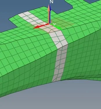
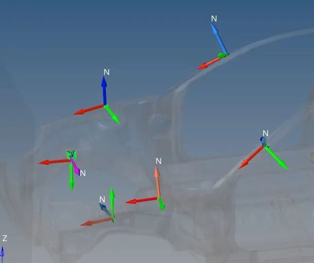
Step-9: Creating an accelerometer. Accelerometers are devices that measure the vibration, or acceleration of motion of a structure. They have a transducer that converts mechanical force caused by vibration or a change in motion, into an electrical current using the piezoelectric effect. In this model, I have created two accelerometers that is placed on the rocker just beneath the B-pillar on either side.

Go to model browser > Right click> Create> Accelerometer
Specify the node where we want this to be placed

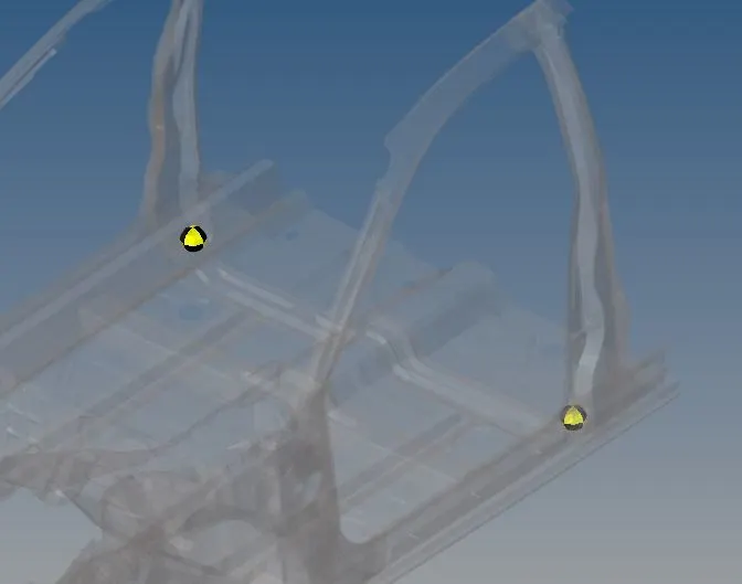
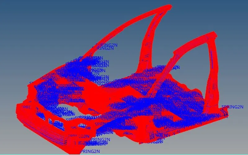
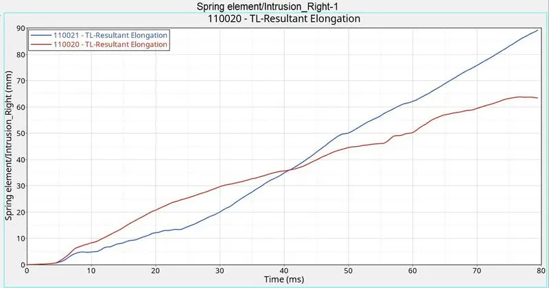
Step-10: Creating springs for intrusions. Calculating intrusion below the dash panel is important because we should know if there will be harm to the driver’s legs. To calculate the intrusions, we must create springs with suitable properties that will help us in plotting its elongation.

Go to 1D> Springs
Select 2 nodes (1 node id is mentioned) to create a spring
Repeat this for the other spring too.
Go to model browser> Right click> Create> property
Rename it as intrusions
Select card image as P4 spring
Put mass 0.01kg and stiffness as 1N/mm. Put the value as 0.001 as that value is in KN/mm.
Go to a component that we created earlier and assign the created property to it.

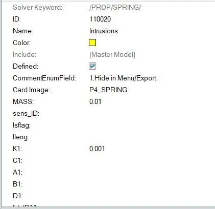
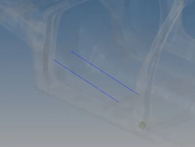
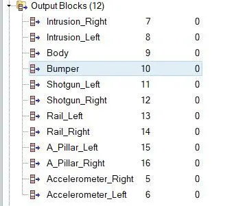
Step-11: Requesting output. By default, the solver gives us some output. But, for the created sections, we must request output from the solver. To keep the process simple, I have deleted the previous TH files.

Go to the solver browser > Right click> TH
Under Th, we have a lot of options. For this project, I have requested INTER output for the Type-7 interface, SECTIO option for all the sections, ACCEL option for accelerometer, and SPRING option for intrusions.
Once we create all these TH cards, we have to select the respective elements for them.
For example, select spring elements for SPRING, accelerometer for ACCEL, and so on.
I have kept the variable as 1 and DEF in every card

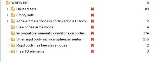
Step-12: Run the model checker. Once our model is set up properly, we must run a final model checker that shows some errors and warnings that will hamper the simulation. The errors displayed in the checker must be dealt with, while the warnings can be ignored.

Go to tools> Model checker > Radioss Block
In the model, checker browser click the green icon on the top right corner to run the checker
I did not come across any errors after running the checker, however, there are 8 warnings that were ignored.

Step-13: Run the simulation.

Go to Analysis > Radioss
Put –nt 4 value in options and hit Radioss to run the simulation

OBSERVATIONS AND RESULTS:

Engine output file

The first thing that we must check to have an idea if the simulation was correct or incorrect is to check out our engine output file. We should check the following things:

Time-step: it should not drop abruptly
Energy error: it should be under -15% on the negative side and not much on the positive side
Mass error: it should be within 1-3%
A message with NORMAL TERMINATION in the end

Incorrect output file:

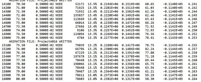
Error that I encountered in the first simulation: I had to run the simulation twice because of a silly mistake on the first try which I understood after reading the engine output file. The energy error was about positive 14-15 % and mass error of about 4-5%. This is a very high value for the error. Such high error values could have meant that there was mass addition in the simulation to prevent time-step from being too small. So, I checked the time-step value which was almost constant at about 5ms and there was no change in this value whatsoever. This was nothing but my imposed time step and it resulted in high error values which meant that this imposed time step was very high. Actually, this value was misinterpreted by me for 0.5ms so I have to change the value from 5ms to 0.5ms and run the simulation again. Comparing both the results, gave me a clear idea of how increasing the time-step decreases the simulation time and reduces accuracy.

Correct output file:

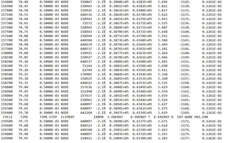
Energy error is in the range of 0 to -2.1% which is acceptable
The mass error starts from 0.9563E-04 and increases till 1262E-02 which is still very less than the 3% maximum error value
The time step is constant throughout the simulation at 0.5ms
NORMAL TERMINATION message is displayed at the end of the file
Total simulation time is about 10664.03s or approx. 3hrs (because of the slow system)

Animation file (.h3d)

The Solver creates n+1 animation files where n is a number of frames. All these animation files are compiled together in one .h3d file. The animation of the frontal crash can be viewed as followed:

Select the drop-down on the toolbar containing the hypermesh icon
Select the Hyperview option to open a new tool
Under load model, browse for the .h3d file and hit apply
Now we can see the animation of the crash

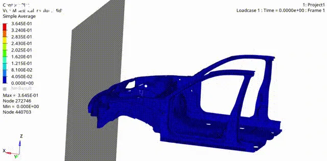
We can also view von mises stress or displacement.

Select the contour option
Select Von mises (or the required option from the dropdown) and hit apply
Now we can run the animation and look at how the stresses develop in the model
Maximum Von Mises stress is 0.3645 GPa.

Time History file (T01)

This file helps us to plot the graph of forces, energies, displacements, accelerations, etc. with respect to the final simulation time in the Hypergraph 2D window.

Select the drop-down on the toolbar containing the hypermesh icon
Select the Hypergraph 2D option
Under the data, file browse for T01 in the simulation folder
Now we can plot the required graphs

Energy plot:

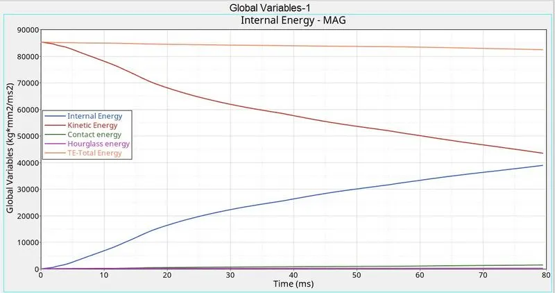
Hourglass energy is 0 throughout the simulation.
Contact energy is also negligible
Kinetic energy starts from its maximum value and decreases over the time suggesting a loss of velocity and energy transfer
Internal energy starts from zero and increases over time as after a crash, the elements start developing resistive forces

Force plots: