Assignment 6 - Frontal Crash-BIW

Frontal Crash-BIW

Aim: To create deck setup, analyse the results with mass balance for frontal crash of car BIW and request for time history plots.

Objective:

1. To check unit system and either follow[Mg mm s] or [Kg mm ms]

2. To create an appropriate interface ,friction 0.2 and recommended parameters.

3. To make sure of no penetrations and intersections.

4. To correct rigid bodies if any issues.

5. To create rigid wall with friction 0.1.

6. To compare the model weight with the full scale 300k nodes model and use added masses to reach target weight 700kg while getting CG about the required range.

7. To create initial velocity 35 mph.

8. To input Time-step :0.5 to 0.1 microseconds and Run 80 ms]

Introduction:

In the proceeding of the study, a piece wise linear model is proposed to represent the vehicle-rigid wall frontal crash. Compared to existing models, this model is developed based on the analysis of crash responses and therefore can reflect the performance of vehicle structures in crashes.The vehicle structure would transmit the impact load in a proper way, i.e. load-carrying path. In addition, there are some weak components arranged as a crumple zone. During the crash, the crumple zone will deform and absorb energy and ensure the rest parts of the vehicle are safe. In the local design, the material and shape of beams, shells and connectors are also considered to achieve better energy-absorbing performance [1].

1) Detailed nonlinear finite element models.

2) Multi body models and multi body based lumped parameter models.

3) Functional approximation or response surface models.

In the proceeding of the study, a piece wise linear model is proposed to represent the vehicle-rigid wall frontal crash. Compared to existing models, this model is developed based on the analysis of crash responses and therefore can reflect the performance of vehicle structures in crashes.the vehicle structure would transmit the impact load in a proper way, i.e. load-carrying path. In addition, there are some weak components arranged as crumple zone. During the crash, the crumple zone will deform and absorb energy and ensure the rest parts of the vehicle are safe. In the local design, the material and shape of beams, shells and connectors are also considered to achieve better energy-absorbing performance [1].

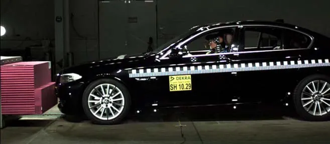
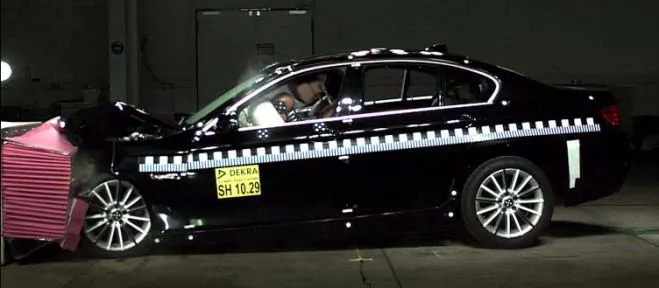
Crash is the explicit analysis. Explicit dynamics analysis is used to determine the dynamic response of a structure due to stress wave propagation, impact or rapidly changing time- dependent loads. Momentum exchange between moving bodies and inertial effects are usually important aspects of the type of analysis being conducted. This type of analysis can also be used to model mechanical phenomena that are highly nonlinear. Nonlinearities may stem from the materials, (hyperelasticity, plastic flows, failure), from contact (high speed collisions and impact) and from the geometric deformation (buckling and collapse). Events with time scales of less than 1 second (usually of order milliseconds) are efficiently simulated with this type of analysis. Based on all these conditions the user will select an explicit solver to solve the analysis. Typical examples of explicit analysis are crash analysis, drop test, bird strike, fan blade out…etc. Obtaining an answer from an explicit simulation can be simple — it can be more challenging to get the correct answer. The predictions of a simulation are usually very difficult to confirm using traditional techniques, making it crucial that the analysis is carried out carefully and thoroughly. Nonlinear analysis requires a lot of experience and a careful understanding of what you want to achieve, as well as a careful understanding of the software's analytical capabilities. When choosing a method for a dynamic problem, considerations must be made regarding the length of time the response can take place compared to the explicit method's stability limit.

Setup Procedure

1. Import the file:

In the data we have two files

1.1. neon_front_0000.rad (starter input file): Which has all data required for the solver such as model information, elements, nodes, loads, boundary condition etc.

1.2. neon_front_0001.rad (engine input file): Which has all data required for the radioss engine i.e speed , time step, run time, what all data we want as output.

To import file,

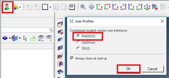
a. change user profile to radioss Because we are using solver as Radioss

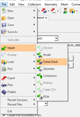
b. File>Import>Solver deck. we can see the new tab where options are available for browsing files. Browse the file FIRST_RUN_0000.rad (starter input file),

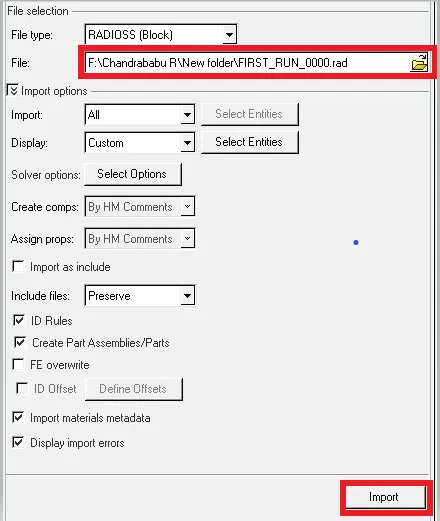
c.Click on import so we can see imported file with required for the solver such as model information, elements, nodes, loads, boundary conditions etc. Show in the fig. 1.1 (both hypermesh and Crash

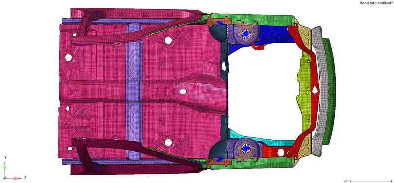
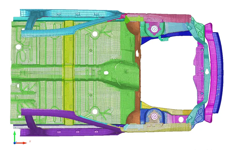
Fig.1.1: Import file

2. Setup for crash: Here some setup are done by Crash and remaining setups are done by Hypermesh.

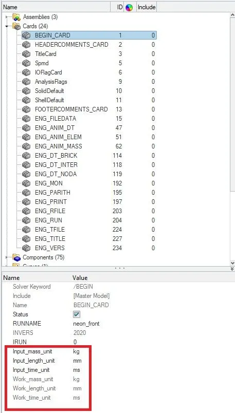
2.1. Check the unit system: To check for the unit system used in the model by clicking on model>cards>BEGIN_CARD it's in Kg-mm-ms.

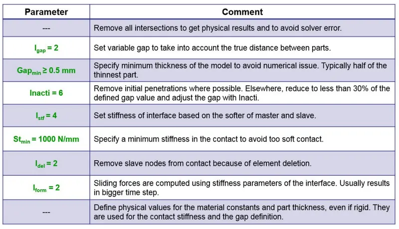
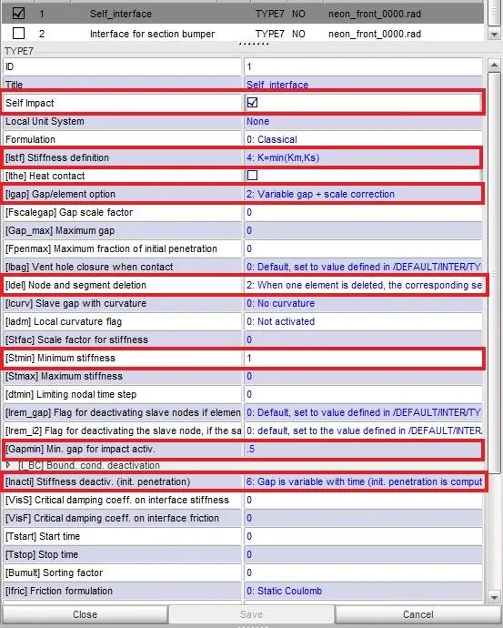
3. Create interface: Here required 2 contact interfaces one is for self interface and other one is to get forces near bumper areas where difficult to create sections. Both interfaces have Recommendations interfaces with gap mim 0.5 and friction 0.2. 0.2.

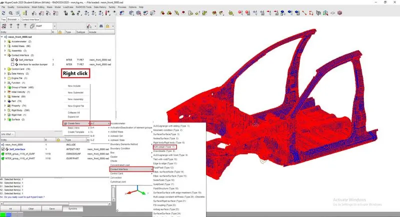
3.1. Self interface: Self interface is created in HyperCrash. To create

a. Right click on tab area>create new > A-c> Contact Interface >Type 7

b. Edit the and apply all Recommendations interfaces. and select the self impact option..

3.2. Interface for Bumper: Similarly create Contact interface. In fig 3.1 shows the both interfaces.

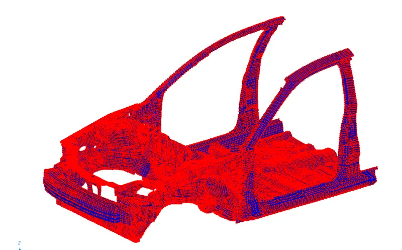
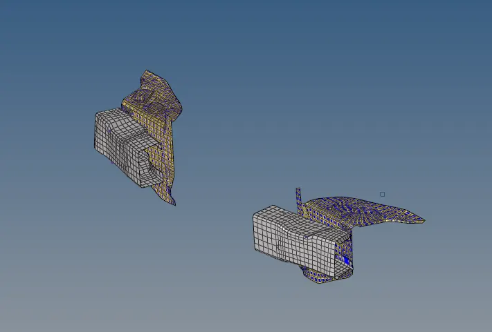
Fig.3.1: Contact Interface

4. Check Initial penetrations and intersection: To check Click on Quality>check Intersection on tree > select parts > click on check penetration. In the figure 4.1 can see the procedure and results

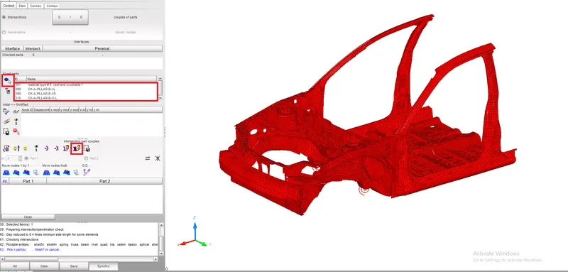
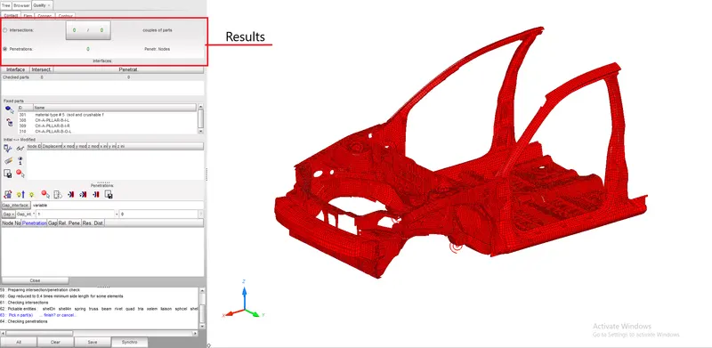
Fig.4.1: Initial penetrations and intersection

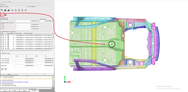
5. Mass Balancing: In order to maintain CG of a car we have to add the mass for missing components. In the given model there are so many parts missing because of the node limit in Student Version.

a. Check CG by Menu > Mass > Balancing > Show CG point. Before adding mass the CG point shown in the figure below

CG point Before Mass adding

b. Add the mass for missing components such as seat, doors, Back seats etc and change the CG point location, and ensure the total mass of car should be 700Kg (Load case > Added mass)

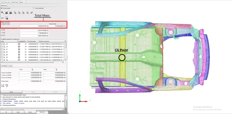
CG point After Mass adding

6. Initial velocity: In order to move the car towards a rigid wall. Given velocity 35mph converts to m/s so we have 15.646 m/s.

a. Right click in tab area > create > I-L > Initial velocity,

b. apply velocity to all components in X direction shown in the fig. below.

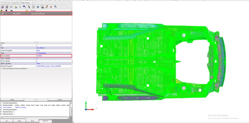
Initial velocity

7. Run Time And Time step:

Input the Run time 80ms that is Final time for the run. in engine cards ENG_RUN

Time step: Time step defaults for all elements which is 0.003ms (Solver > Create > Engine keywords > DT >DT) . If the time step of a simulation reaches ΔTmin">ΔTmin , then the following actions will happen depending on which element type is controlling the time step. For /BRICK or /QUAD elements, the simulation stops and a restart file is created. For /SHELL or /SH_3N elements, the element controlling the time step is deleted from the simulation. For all other element types, ΔTmin">ΔTmin is not used.

8. Create rigid wall: Create Rigid wall by Solver > Create > Rwall > Plane.

Give sliding with friction of 0.1.

Search distance 2000 (Distance for slave search).

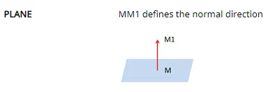
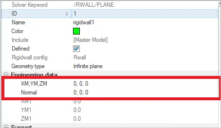
XM, YM, ZM is the location where we need Rigid wall

Normal is the direction normal to the rigid wall depending on the Global coordinate system. here we need normal in X direction.

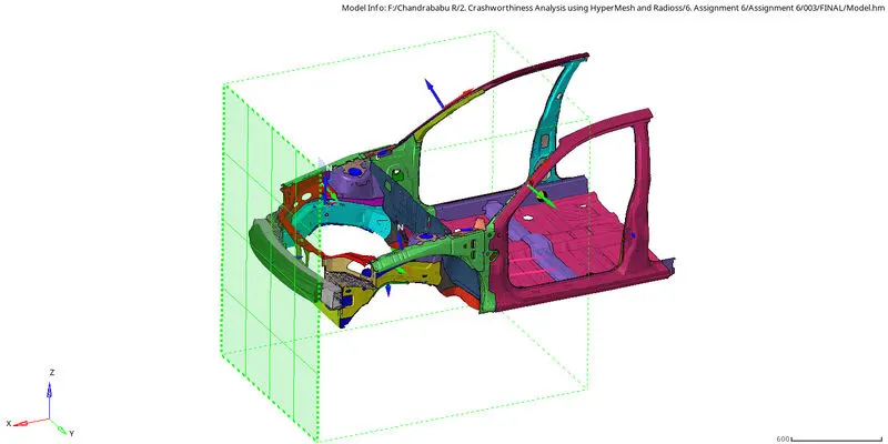
Rigid Wall

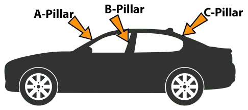
8. Create Sections: Sections are created in components to get the exact forces at a particular section. Total 6 sections are required. rails from bumper, Shotgun cross section and A pillar cross section for left and right side.

To create a section, we need to define a moving frame.

Create a moving frame: Use the Systems panel to create rectangular, cylindrical and spherical coordinate systems. Use this function when you want to define nodes, loads and constraints in a different coordinate system. the following steps to create moving frame by Create by Node Reference Sub panel

a. Solver > frame > mov

b. Select the coordinate system type you want to create.

c. Select the node that defines the origin by selecting it in the modeling window, or by entering the node ID.

d. x-axis node: Select the node that defines the x direction by selecting it in the modeling window, or by entering the node ID.

e. xy-plane node: The following Output requests are asked in the given problem.Select the node that defines the xy plane by selecting it in the modeling window, or by entering the node ID.

f. relative size: Specify how large, in model units, systems are displayed relative to the model size.

In fig. 8.1 shows the moving frame

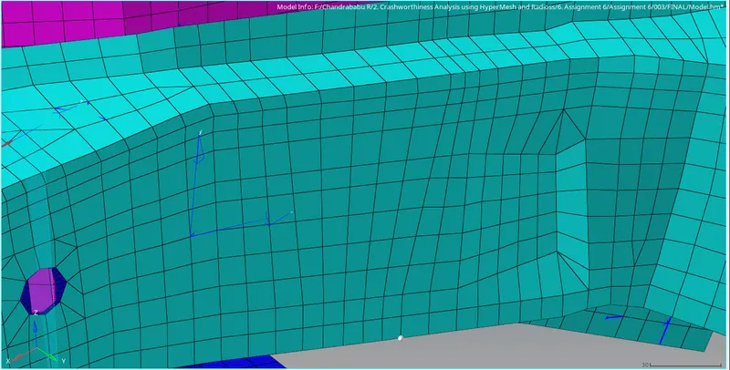
Fig.8.1 Moving Frame

Create Section: A section is a set of nodes and a set of elements. A section is a cut in the structure, where forces, moments or energy will be computed and stored in output files (using /TH/SECTIO). In Radioss /SECT, /SECT/PARAL and /SECT/CIRCLE can be used to define a section.

Generally, to define the section, the following points are required:

a. A cutting plane (which defined either by 3 points or by parallelogram or by a circular disk)

b. A reference point to compute forces

c. A direction of the section

d. In /SECT, the cutting plane is defined by a group of elements and its orientation by a group of nodes.

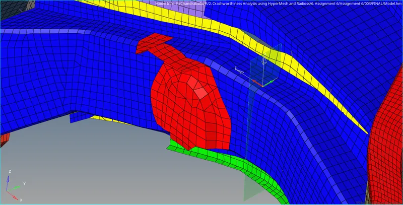
Review the section by pressing 'Q'

Similarly define all the sections shown in the figure 8.2

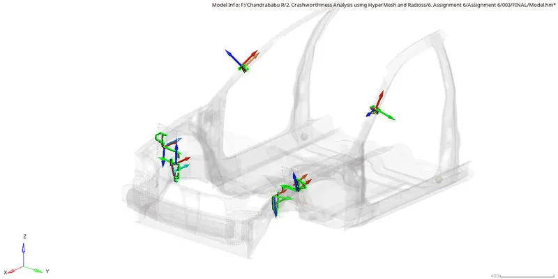
Fig.8.2 Section

9. Create accelerometers: Defines accelerometers using a node and skew system.

Solver > ACCEL > Select node And create

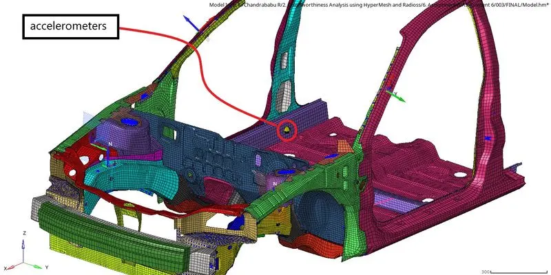
In the figure 9.1 Shows the complete Setup model and ready for simulation.

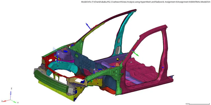
Fig.9.1: Complete model

10. Output requests: In output requests we are going to request all required output which we need. To request Solver > Create > TH > select things to record in result.
1. Sectional force in the rails at the location of indicated node 174247.

2. Axial force received on the rails from the bumper.

3. Shotgun cross sectional forces.

4. A pillar cross section.

5. Acceleration curve received on the accelerometer at base of B pillar (on B pillar rocker).

6. Intrusions on the dash wall 66695,66244.

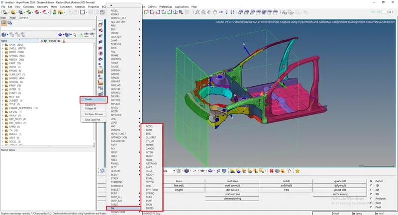
Run simulation Analysis > Radioss

Simulation Results:

In fig 10.1 shows the simulation for Frontal crash of car BIW.

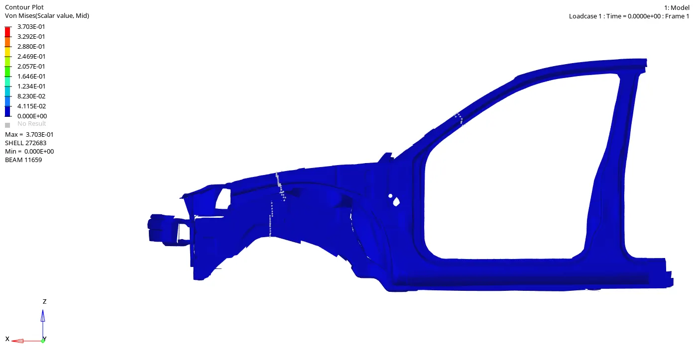
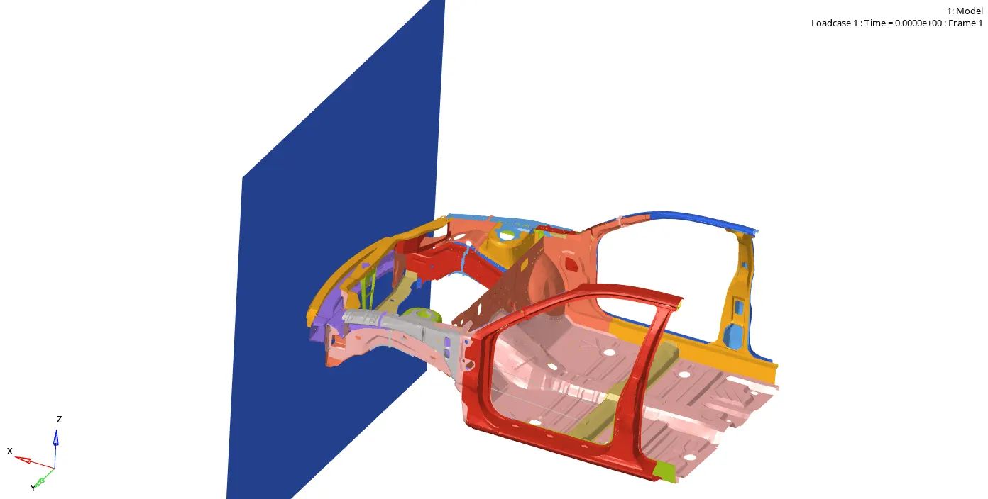
Fig. 10.1: Frontal Crash

From the simulation we can see that. Initially the bumper starts crushing then the bumper forces are transferred to the left and right rail From the rail forces are transferred to A Pillar LH and RH. In each stage the forces are going to reduce because energy is absorbed in each stage. Because of no engine blocks, suspension system etc the car BIW is going to go down at the end of simulation. In the fig 10.2 shows the stages.

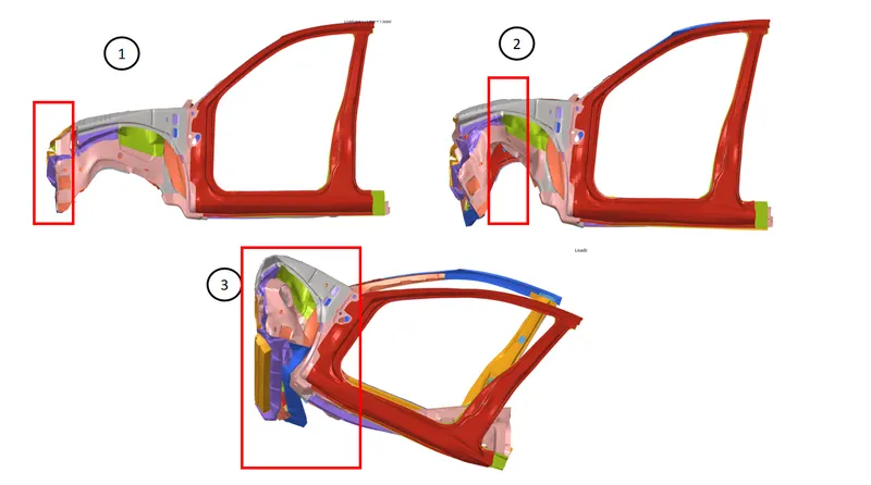
Fig. 10.2: Frontal Crash Stages

Load-carrying Path and Crash Process: Generally, vehicles have a high relative velocity in the crashes. For this reason, the frontal structures always have enough space for the crashworthiness design. In many vehicles, there are three paths to transmit the impact load.

1. Path1: Accessories - Front bumper and Crash box - Front longitudinal beam-Engine - Firewall

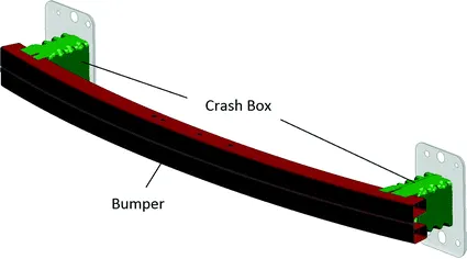
2. Path2: Upper wing beam - A pillar - Guard beams of door

3. Sub-frame - Sill beam

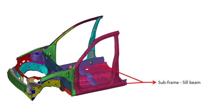
For most cases, the first path affords more than half of the total energy in crashes. Accordingly, the ideal crash process contains several stages.

11. Graphs:

11.1 Energy: Energy, in physics, the capacity for doing work. It may exist in potential, kinetic, thermal, electrical, chemical, nuclear, or other various forms.

In FEA we have Total Energy, Internal Energy, Kinetic energy, Contact energy and hourglass energy

Total Energy (TE): Total Energy is the sum of Internal Energy, Kinetic energy & External Work

Internal Energy (IE): The internal energy of a thermodynamic system is the energy contained within it. It is the energy necessary to create or prepare the system in any given internal state. It does not include the kinetic energy of motion of the system as a whole, nor the potential energy of the system as a whole due to external force fields, including the energy of displacement of the surroundings of the system. It keeps account of the gains and losses of energy of the system that are due to changes in its internal state

Kinetic energy (KE): In physics, the kinetic energy (KE) of an object is the energy that it possesses due to its motion. It is defined as the work needed to accelerate a body of a given mass from rest to its stated velocity.

Contact energy (CE): Contact energy is the energy acting opposite to the system to prevent the penetration acting on the system due to applied load case.

Hourglass energy (HE): This is usually done by adding extra stiffness or viscosity across the diagonal which adds extra strain energy into the system and we call this as Hourglass Energy.

Energy Errors:

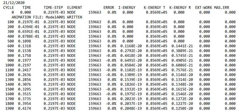
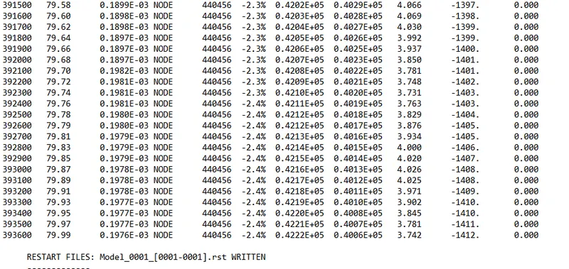
Energy error is 0 to -2.4 % and mass error is 0% this is due to energy being dissipated from the system. In case of under integrated elements, the Hourglass Energy can explain a negative Energy Error since it is not counted in the energy balance.

Results:

11.2. In a frontal crash we have the following energy graphs.

1. Initially car is at rest so there is no any energies, once car moving with velocity of 15.646 m/s towards rigid wall for frontal crash with maximum KE and IE of 85686.8 `(Kg-mm^2)/(ms^2)`

2. When a car is hitting the rigid wall the velocity of every part is going to drop w.r.t to time with different magnitude which is dependent on the distance from the rigid wall. shown in the fig. below.

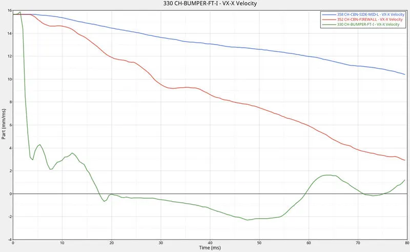
3. Initially IE is zero and it's increasing w,r,t to time until the complete crash happens. because at the initial stage we have maximum velocity,Kinetic energy is directly proportional to the Velocity. so kinetic energy is max at initial stage after hitting the KE is observed by plate so internal energy increase until the component reaches complete crash after that there is no energy observed (internal energy ΔU = q+w)

We have Total Energy = Internal Energy + Kinetic energy + External Work, Here TE is not depending on external work because there is no any force acting on the car BIW only the car is moving with velocity.

as IE increases and KE decreases in the same path so the TE remains Constant. TE is slightly decreasing because of Contact energy i.e Contact energy is the energy acting opposite to the system to prevent the penetration acting on the system due to applied velocity.

4. Hourglass energy is constant because both are controlled by element formulation. Here hourglass is controlled by Physical stabilization i.e changing material level in ISHELL is 24 QEPH Shell formulation

In the fig. 11.2 shown energy graph

In the fig. 11.2 shown energy graph

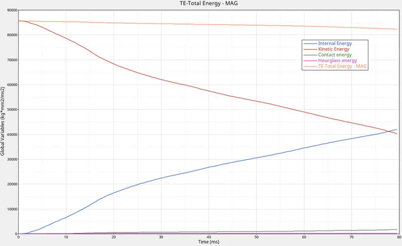
Fig. 11.2: Energy Graph

From the graph we have

a. KE max= 85686.8 Kg-mm^2/ms^2 at time 0 ms.

KE min= 40331.3 Kg-mm^2/ms^2 at time 79.5 ms.

b. Internal energy max= 41986.8 Kg-mm^2/ms^2 at time 79.5 ms^2

Internal energy min= 0 Kg-mm^2/ms^2 at time 0ms^2

c. Contact energy max= 1733 Kg-mm^2/ms^2 at time 79.5 ms^2

d. Hourglass energy max = 228 Kg-mm^2/ms^2 at time 79.5 ms^2

11.3 Rigid wall forces: Rigid wall forces are the reaction forces for the applied forces.

1. Initially The rigid wall forces, once the car BIW with velocity 15.646 m/s reaches rigid wall its start producing the reaction forces, in graph we can see there is sudden increasing of rigid wall forces due to bumper touching to rigid wall and it decreasing until bumper and crush tube getting max deformation.

2. R-wall forces are increasing to max (134.98KN) value when all the forces are transferring to RH and LH rail, once rails start deforming, Rwall forces are decreasing because Rails are absorbing energy. also velocity decreasing due to decreasing velocity the rigid wall reactions forces are decreasing.

3. Remaining energy absorbed by A pillar and Still beams, we can see less Rwall forces are dropping down because velocity dropping shown in the fig 11.3.

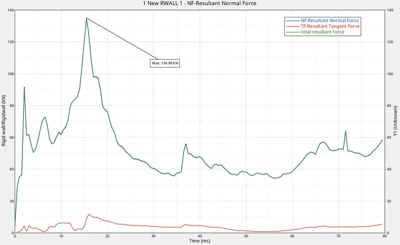
Fig. 11.3: Rigid Wall forces.

11.4. Forces At Sections: Here we are going to review the Load-carrying Path and forces at particular section, we have total 6 sections. 3 are in LH side and 3 are in RH Side.

11.4.1. Axial force received on the rails from bumper: Force which is coming from the crush tube and bumper is received by rails. to find this force we have a contact interface b/w crush tube and rail. This force is divided into RH and LH interfaces. in fig. 11.4.1 shows the force graph for LH & RH Rail.

a. Force received at RH rail is 17.464KN @ 4 ms

b. Force received at LH rail is 16.45KN @ 9 ms

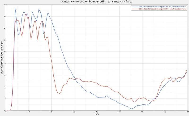
Fig. 11.4.1: Axial force received on the rails

11.4.2. Sectional force for rails: From the bumper part of load will carry through LH & RH rails of the car. We have a section for the same. in fig. 11.4.2 show the Sectional force for rails. From the graph the max forces are flowing through the rails because the rail is more stiffer compared to the bumper and crush tube.

a. Force received at Rails Sectional RH is 41.41KN @ 15.5 ms

b. Force received at Rails Sectional RH is 34.143KN @ 16 ms

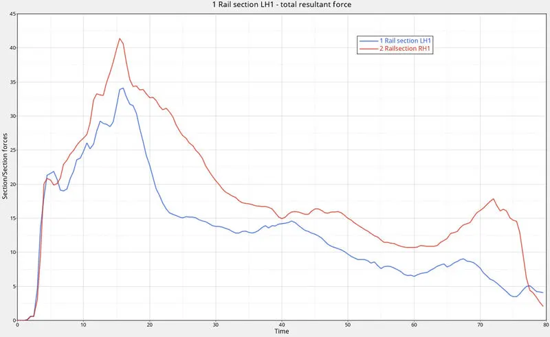
Fig. 11.4.2: Sectional force for rails

11.4.3. Shotgun sectional forces: From the bumper part of load will carry through LH & RH shotgun of car. We have a section for the same. in fig. 11.4.3 show the Sectional force for Shotguns. From the graph the force flowing through the Shotguns is less than Rails because less stiffer and from the structure design we can see the distribution is more on rails than the shotgun.

a. Force received at Shotgun section RH is 10.97KN @ 37 ms

b. Force received at Shotgun section LH is 19.1559KN @ 76 ms

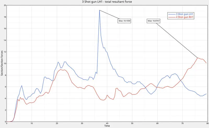
Fig. 11.4.3: Shotgun sectional forces

11.4.4. A pillar cross section: From the Shotgun load will carry through LH & RH A Pillar car. We have a section for the same. in fig. 11.4.4 show the Sectional force for A pillar. From the graph the forces are flowing though the A pillar is less then Rails and Shotgun because less stiffer and from the structure design we can see the distribution is more on rails then the shotgun then A pillar.

a. Force received at A pillar section RH is 5.69 KN @ 69 ms

b. Force received at A pillar section LH is 21 KN @ 3.78 ms

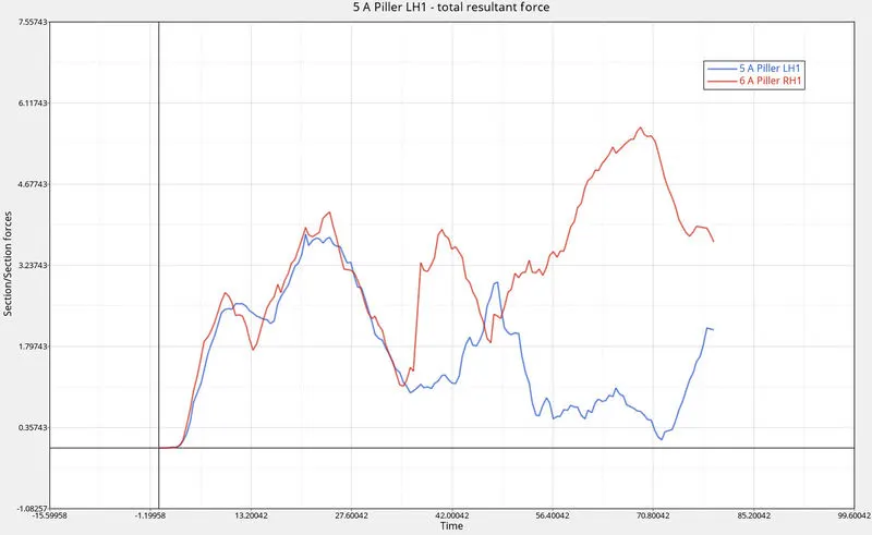
Fig. 11.4.4: A pillar cross sectional forces

All Right side and left side graphs are shown in fig. 11.4.5 and 11.4.6

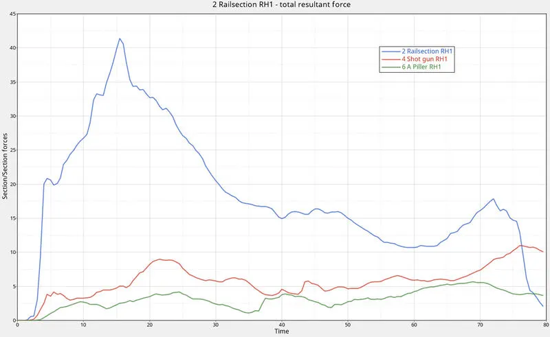
Fig. 11.4.5: RH Force Distribution

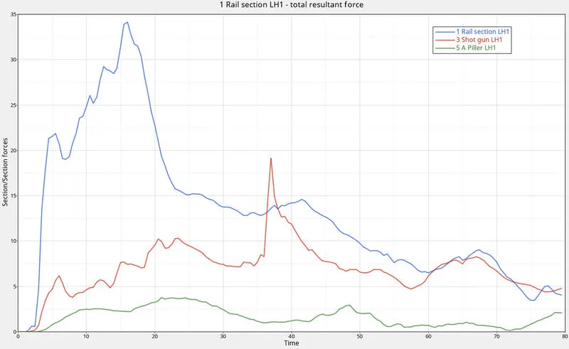
Fig. 11.4.6: LH Force Distribution

From the both graphs one can say the loads are flowing as per requirement. forces at distribution is Rails > Shotgun > A Pillar.

11.5. Acceleration curve received on the accelerometer at base of B pillar (on B pillar rocker): Vibration is most commonly measured using an accelerometer. An accelerometer is a sensor that measures the dynamic acceleration. The benefits of an accelerometer include linearity over a wide frequency range and a large dynamic range.

is used to measure the change in velocity wrt time so that sudden impact or crash we can check change in velocity of particular node. In the fig. 11.5 we have an accelerometer graph. Initially there is no change in velocity ie acceleration. Its starts fluctuating due to impact, due to impact the velocity is dropping w r t time.

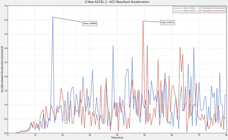
Fig. 11.5: Accelerometer Graph.

11.6. Intrusions on the dash wall 66695,66244 : Intrusion is change in space or decreasing length horizontally of the car driver compartment. so due to Intrusions we can say safety of the driver. intrusion is measured by creating spring elements with less mass and stiffness so the one can check spring compression, from compression will give change in length of spring. in the fig. 11.6 shows the graph for spring compression as Intrusion.

from graph we have -74.55mm and -82.94mm Intrusions i.e 10-11%

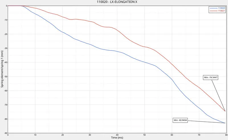
Fig. 11.6: Intrusions Graph.

Conclusion: The overall objective of the work was to simulate a Frontal crash-test and validate the results of the simulations obtained from the crash-test. Simulation was performed using the Radioss software package.

he graphical results obtained all showed that the test models behavior were shown.

Due to the limited number of nodes in the student version some of the biw, engine blocks, suspension system etc are removed, so results are not as in real condition.

It has been observed that there is minimum deformation of the cabin and also there was minimum intrusion at given nodes in the driver compartment.

References

[1] A MODEL OF VEHICLE-FIXED BARRIER FRONTAL CRASH AND ITS APPLICATION IN THE ESTIMATION OF CRASH KINEMATICS, Zuolong, Wei Hamid Reza, Krimi Kjell Gunnar, Robbersmyr University of Agder Norway Paper Number 15-0161