Frontal crash of a car using Crashworthiness analysis on Radioss, Hypermesh

Aim:

To perform the crash analysis on the frontal section of the car and to check where the stresses are acting on it.

Objective:

The main objective is to do as the instructions.

1. To check the unit systems and change if necessary
2. Create an interface of Type 7 with the friction value of 0.2 and other parameters.
3. Making sure there aren’t any penetrations
4. Correct rigid bodies for any issues
5. Create a rigid wall with friction 0.1.
6. Compare the model weight with the full-scale 300k nodes model and use added masses to reach the target weight of 700kg while getting CG about the required range.
7. Give an initial velocity of 35 mph.
8. Use a model checker to ensure good quality.
9. Give the Time-step: 0.5 microsecond.
10. Give Run time as 80 ms.

Tasks to complete:

1. Add a Cross-Sectional force in the rails at the location of indicated node 174247.
2. Add axial force received on the rails from the bumper.
3. Add cross-sectional forces on Shotgun.
4. Add a cross-section a pillar.
5. Acceleration curve received on the accelerometer at base of B pillar (on B pillar rocker).
6. Add Intrusions on the dash wall 66695, 66244.
7. Plotting the graph for the energies.

Methodology:

The Methodology is for the given frontal part of the car is as follows:

1. Opening the File.
2. Checking the dimensions.
3. Creating the Interface.
4. Creating the Rigid Wall.
5. Creating a COG point.
6. Creating the Initial Velocity.
7. Performing the check for errors.
8. Giving the Time-Step and Run time Values.

Theory:

Frontal area:

The frontal area of the car is called the crumble zone. It is so-called as it is the only part which gets collided(in most cases) with the other vehicles in case of crash. The frontal area should be created based on the aerodynamic drag since it faces the air head-on. The total resistance of a vehicle is the product of the frontal area and the drag coefficient. The force exerted by air on anybody moving through is aerodynamic drag. A good aerodynamic shape is known to be a narrow edges to gradually increasing edges but that’s a fallacious fact. The good aerodynamic shape is a curved part but with a blunt on the windward side and gets slender on the leeward side.

Procedure:

1. Opening the File:

• To Open the Starter (_0000.rad) file, Go to the File menu in the Standard menu bar >> Click Import >> Click Solver Deck >> Select the file to open >> click Import.
• The model is displayed in the Graphics Area.

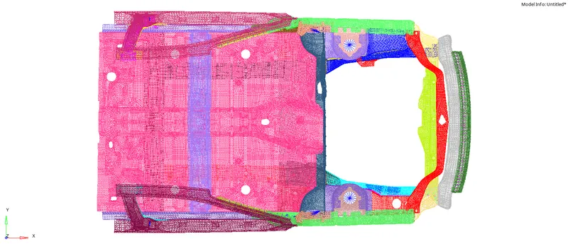
2. Checking the Units:

• Once the file is opened the dimensions should be checked.
• The unit system can be checked using the cards section.
• Go to the Model Browser >> Click Cards >> Click BEGIN_CARD >> In the Entity Editor Tab check for the Input mass, Length, time units.

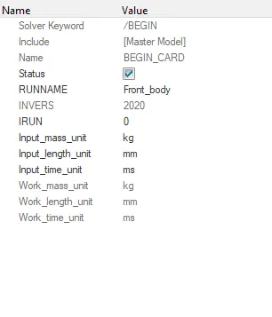
• The unit followed for the project is “Mass (Kg), Length (mm), and Time (ms)”

3. Creating the Interface:

• The Interface for this project is TYPE 7 type of interface. The Details on TYPE 7 is cleared in the Terms used Section.
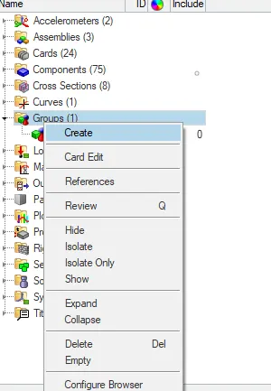
• To create a new interface. Click on the Groups tab in the Model Browser >> Right-click on it >> Click Create >> Give the Name as TYPE 7 >> In the Entity Editor, Select the Card image as “TYPE 7” >> Select the Slave entities as components and select the component >> Select the Master Elements and Select as components and select the components >> Give the values of Istf(stiffness definition) as 4, Igap (gap/element option) as 2, Idel (Nodes and segment deletion) as 2, Irem_gap (Deactivating slave nodes if element size is lesser than gap value, in case of self-impact contact) as 2, Irem_i2 (deactivating the Slave node, if the same contact pair/nodes have been defined in interface type 2) as 0, stfac (Stiffness or scale factor) as 2, Fric (Coulomb Friction) as 0.2, Gapmin (Gap for impact activation) as 0.5, Inacti (Deactivation of stiffness) as 6, Iform (Stiffness or viscous formulation) as 2.

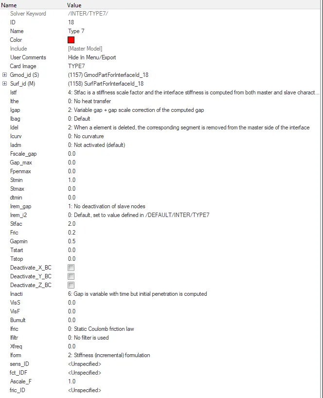
• The Card is created.

4. Creating the Rigid Wall:

• To create the Rigid Wall, the Solver browser needs to be opened.
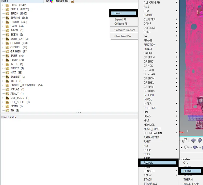
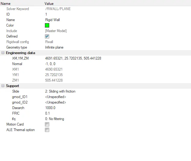
• In the Solver Browser, Right-click on the tab area >> click on the RWALL >> select PLANE >> A new rigid wall card is created. Give a name to it >> Select the Geometry Type as “Infinite Plane” >> Click on the “XM, YM, ZM” (X, Y, and, Z Coordinates of Base node M) >> Select the node at the plane the rigid wall needs to be created >> Select the Normal around the axis and based on the direction of the normal give a ‘-’ sign based on it. >> Give the Slide value as 2, Dsearch value as 1000, Fric Value as 0.1.

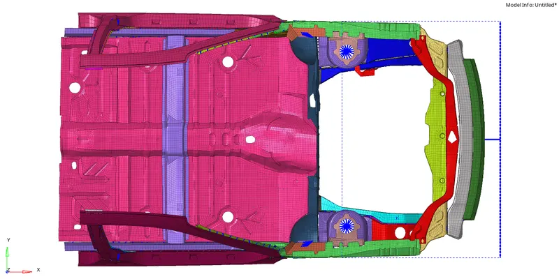
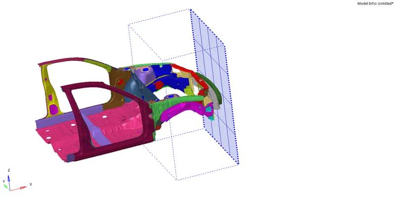
• The Rigid wall is created.

5. Creating a COG point:

• The COG point is created based on the mass.
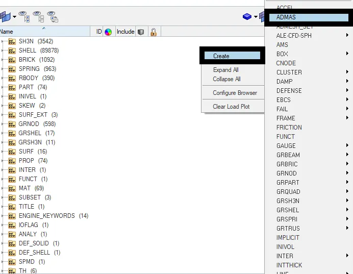
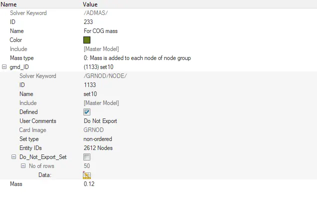
• In the Solver Browser, Right-click on the Tab area >> Click on the ADMAS >> a new mass card is created >> Give a name to it >> in the Entity Editor, Select the Mass type as 0 >> Select the group by right-clicking on the gmd_ID >> click create >> select the nodes at which the mass needs to be added >> give the Mass value.

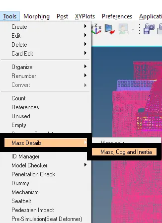
• Check the COG coordinates in the Tools menu >> Click on Mass Details>> Click Mass, COG, and inertia. >> A new dialog box opens >> click on COG >> Check the coordinates of COG and copy the coordinates.

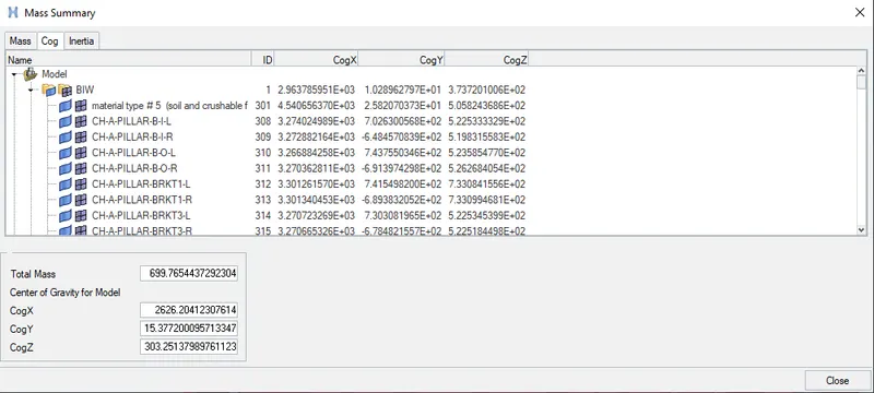
• To create a new COG point, In the Geom panel, Select nodes option >> Give the Coordinates >> Click create.

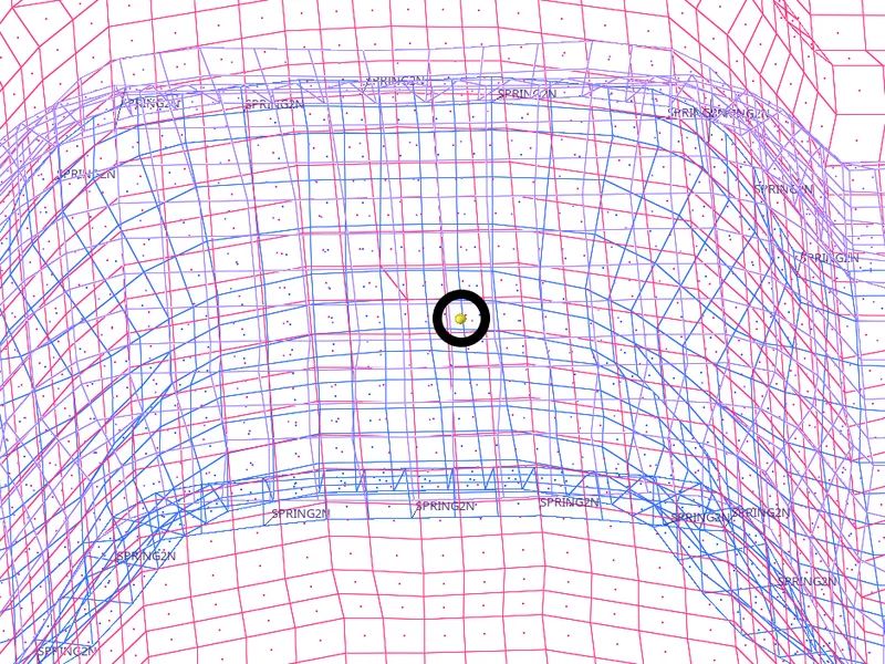
• A new COG node point is created

6. Creating the Initial Velocity:

• To create the Initial Velocity, In the Solver Browser, Right-click on the Tab area >> Click on Boundary Conditions >> Select INIVEL option >> Give a name to the card >> right click on the gmd_ID option >> click create >> Select the nodes as displayed and click proceed >> Give the Velocity value as 15.64 >> Select the coordinate at which direction the velocity needs to be added.

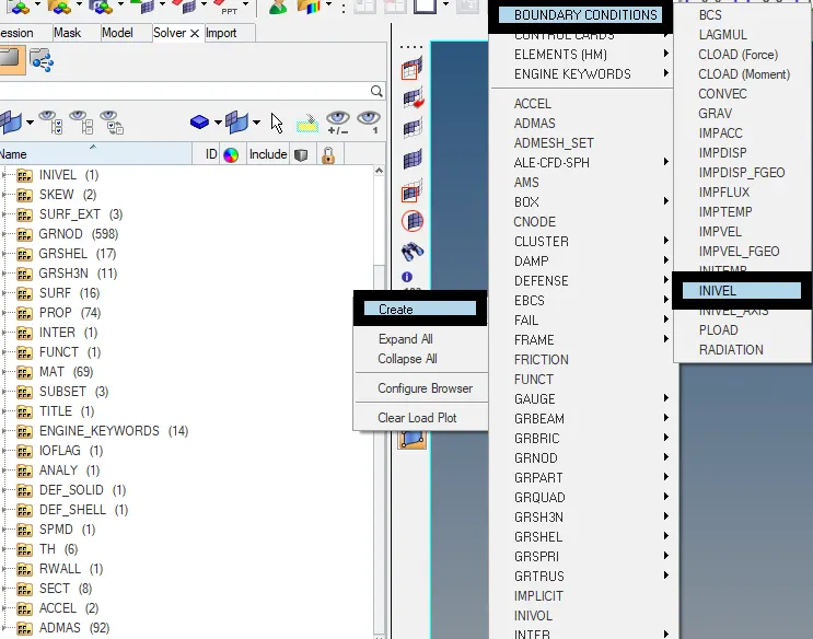
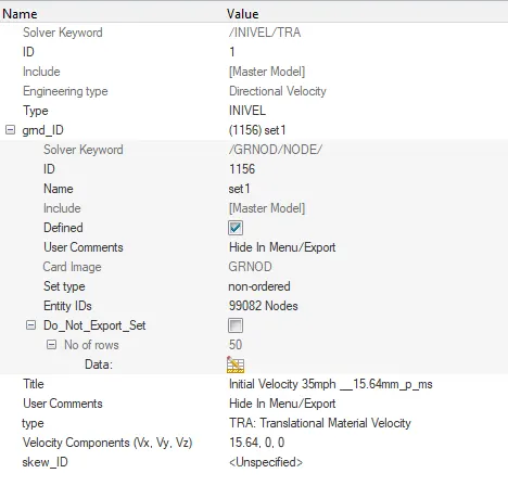
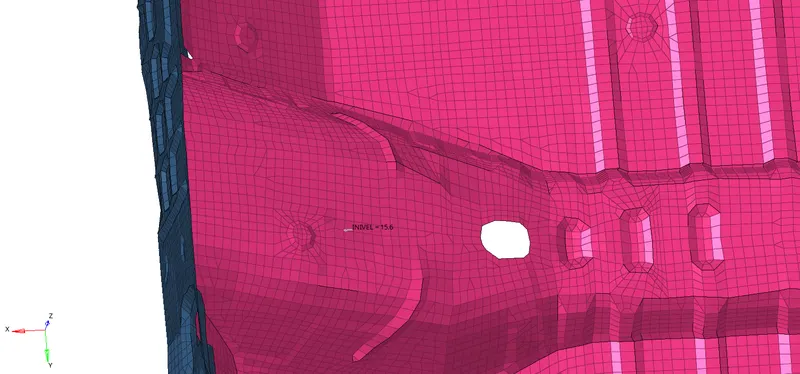
• Given initial velocity value as 35mph (miles per hour). We need to convert the given value into the selected unit system.
• we know 1 mile = 1.609mm and 1 hr = 3.6 ms

`v_0 = (35 xx 1.609 xx 10^6)/(3.6 xx 10^6)`

`v_0 = 15.64 (mm)/(ms)`

• The Value of initial velocity is converted from mph to mm/ms.

7. Performing the check for errors:

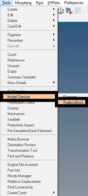
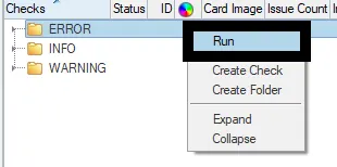
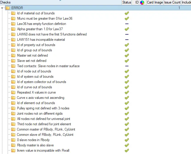
• To check for the errors, go to the Tools menu >> click on the Model Checker >> Select Radioss Block >> In the Tab area, a new Browser opens >> on Errors, Right-click and Click on run all >> Check for the Errors ( Errors are generally noted as a cross mark) >> clear the errors.

8. Check for the penetrations:

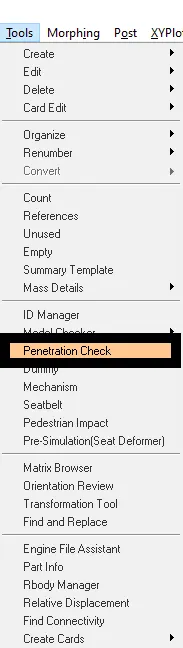
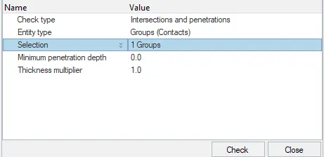
• To check for penetrations, go to the Tools menu >> Click on the Penetration check >> In the Entity Editor, click on Selection and click on group >> give the group. In the Tab area, the penetrations are checked.
• There are no penetrations in the model.

9. Giving the Time-Step and Run time Values.

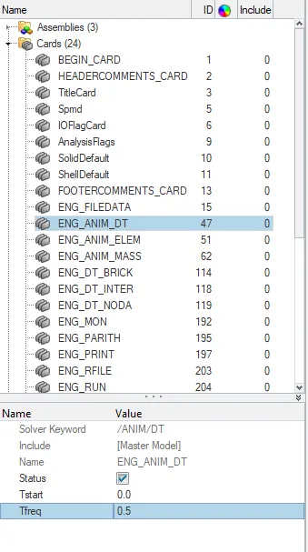
• To give the Time Step value, Go to the Cards >> Click on the ENG_ANIM_DT >> In the Entity Editor, Give the Tfreq value as 0.5.

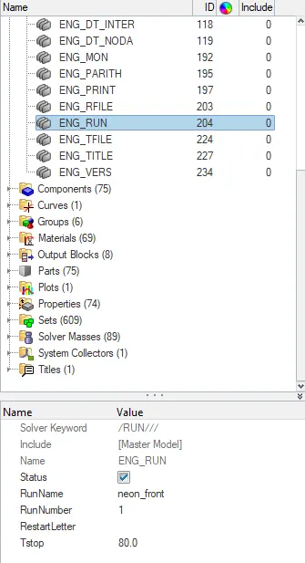
• To give the Run time Value, In the cards >> Click on the ENG_RUN >> In the Entity Editor, give the Tstop value as 80.

10. Creating the Sections:

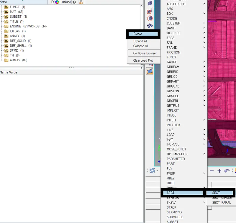
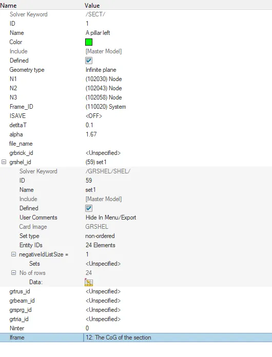
• To create the cross- section, open Solver browser >> right click on the Tab area >> Click Create >> Click SECT >> Click SECT in the sub panel of sect option >> In the Entity Editor, Give the N1, N2, and N3 values >> a skew is created >> right click on gmod_id and click create >> Click on Entity IDs and select the nodes to create a section >> Give the deltaT value as 0.1 and alpha value as 1.67 >> select the grshel_id by right clicking on it >> select the elements on the area to create the section >> Give Iframe values as 12.

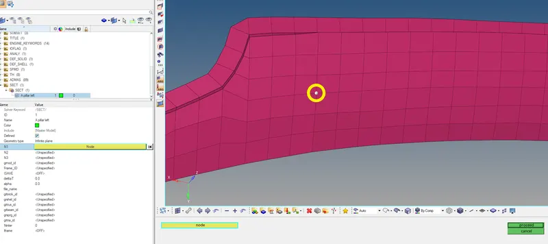
• The Frame is created to make local coordinates of the section.
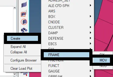
• To create the Frame, Right Click on the Tab Area in the Solver Browser >> Click Create >> Click FRAME >> Click MOV >> Select the nodes so create an axis >>click Create.

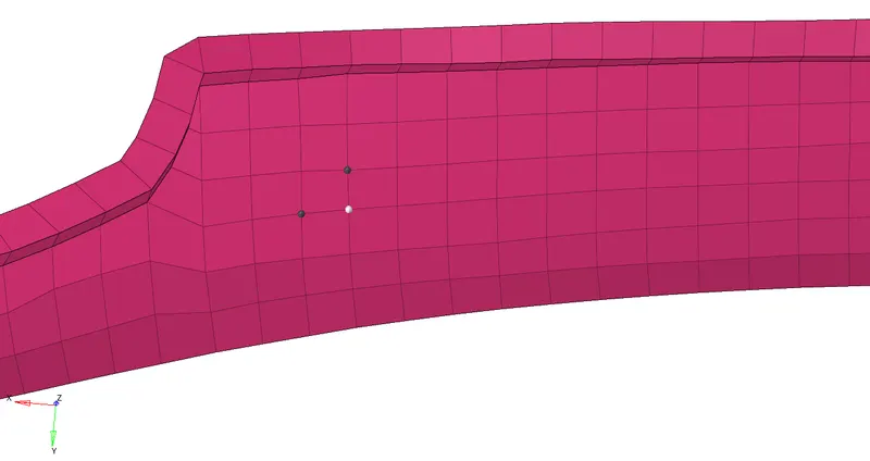
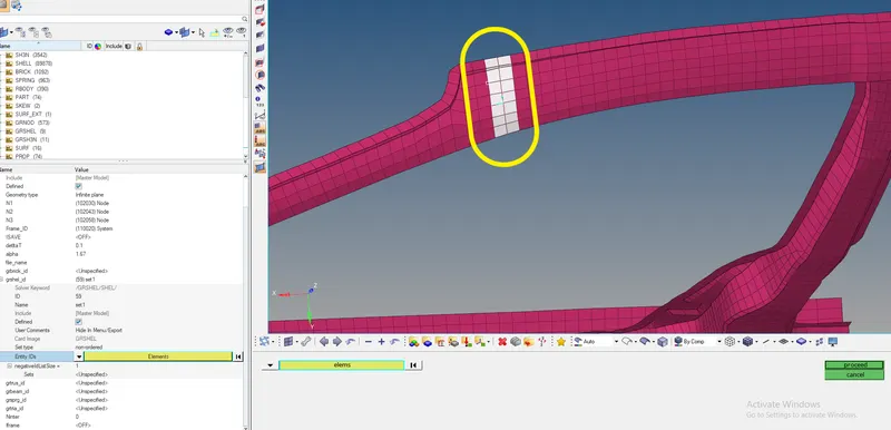
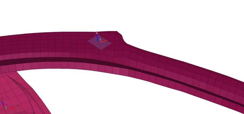
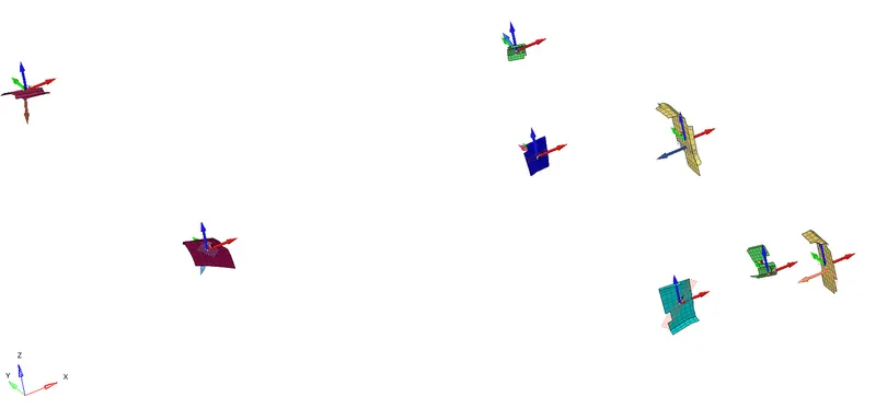
• The Section is created. The cross-sections for the parts are similar and can follow the same procedure.
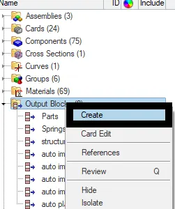
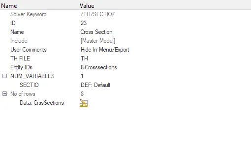
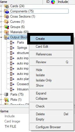
• The section which is created needs to be called and therefore, to call the sections, Go to the Model browser >> Right-Click on the Output Blocks >> click create >> give a name to the card as Crossections >> Select the Entity IDs with the cross-sections and selection of the cross-sections is done.

11. Creating the Accelerometers:

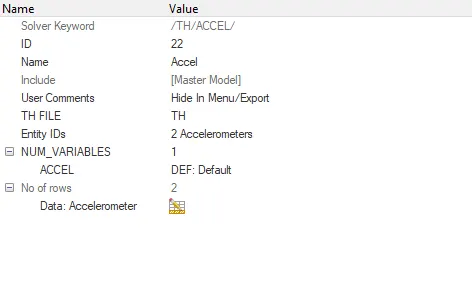
• To create the Accelerometers, open Solver Browser >> Right click on the Tab area >> Click create >> Click ACCEL >> select the node as specified location above >> give the Fcut value as 1.65.

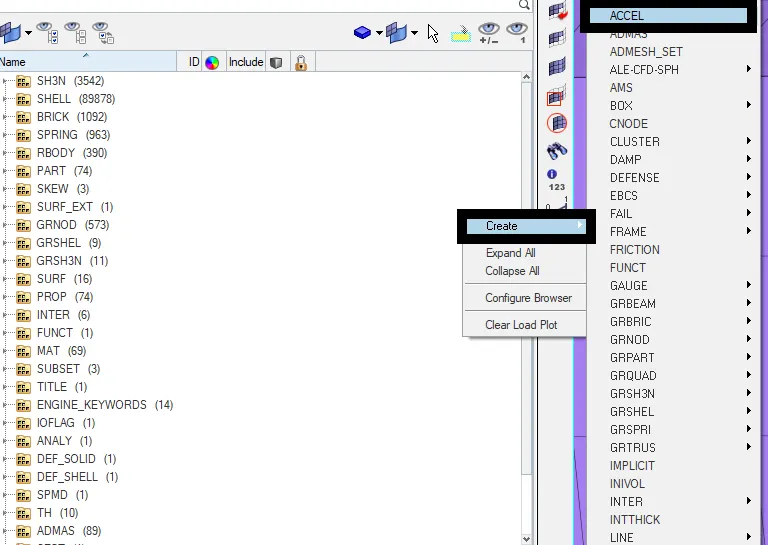
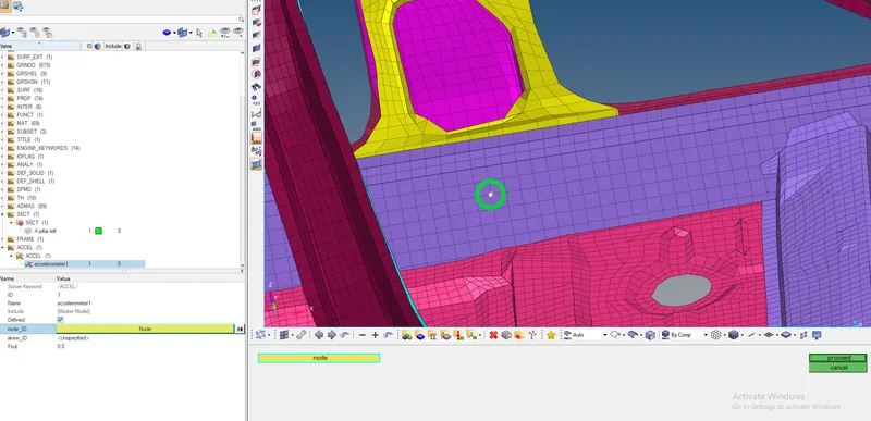
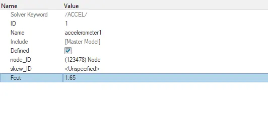
• The accelerometers are created and to call the accelerometers the following steps are created.
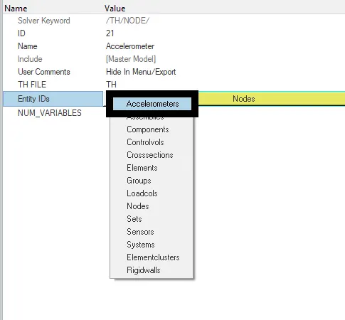
• The card which is created needs to be called and therefore, to call the accelerometers, Go to the Model browser >> Right-Click on the Output Blocks >> click create >> give a name to the card as accelerometers >> Select the Entity IDs with the accelerometer and selection of the accelerometers is done.

12. Creating the Intrusion:

• To create the intrusion, select the node at which the intrusion can be checked.
• Go to the Tools panel >> Click on numbers >> Select the nodes >> click on ID >> give the node id as specified (given 66695, 66244) >> Click on display.

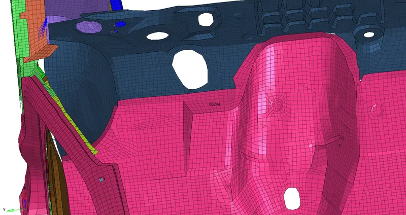
• The node number is displayed.
• Now go to the Solver Browser >> right click on the tab area >> click create >> click SKEW option >> select MOV option >> give a name to it >> select the nodes ( origin, axis, Plane nodes)
• The coordinates are created.

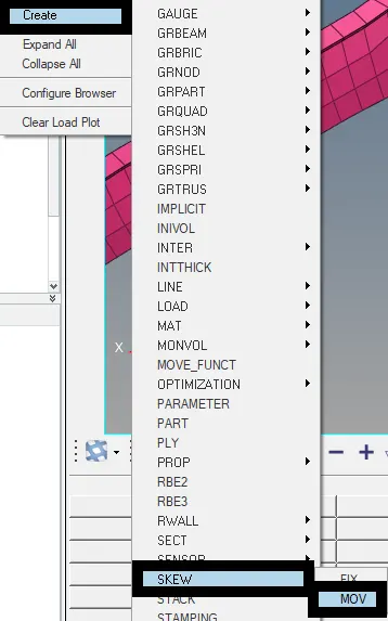
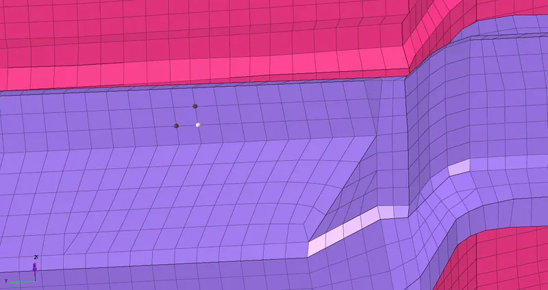
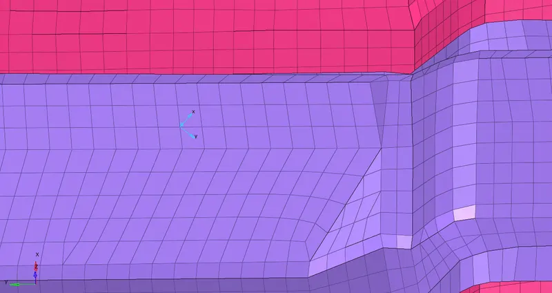
• The card which is created needs to be called and therefore, to call the Intrusion, Go to the Model browser >> Right-Click on the Output Blocks >> click create >> give a name to the card as Intrusions >> Select the node (The number to which the number is displayed) >> Select the System (the Skew coordinates created).

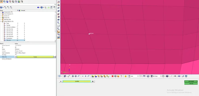
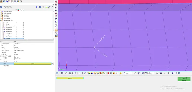
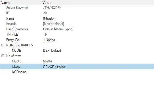
• The intrusion is created and called.

13. Creating the Animation:

• To create an animation, Go to the Hyper View in the Client Selector. >> Hyper view is opened>> Select the File to view the animation (Note: File is in .h3d format in the respective case folder) >> Click Apply.
• The animation is opened and it can be seen by clicking play in the Toolbar.

14. Plotting the Graph:

• To plot the graph, go to the Client Selector option in the Tool Bar >> Change it to HyperGraph 2D >> The HyperGraph is opened >> Select the Data File from the respective folder >> Select Cross-sections, Parts > Internal Energy, Kinetic Energy, Total Energy, Hourglass Energy, Contact Energy > MAG >> Click Apply.
• The method is the same for the other cases.
• The Plots are created.

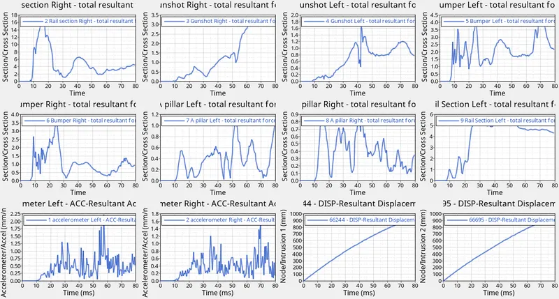
• The graph above shows all the Intrusions, Accelerations, and Cross-sections of the car.

Errors faced:

The Errors faced during the project are while running the simulation the dialog box shows errors though there were no errors while checking in the Model Checker. The Errors can be seen using the Hyper Crash the hyper crash helps us find the errors and clear them.

To open Hyper crash, Go to the Application Tab in the Standard tools menu >> Click Hyper Crash. The Hyper Crash opens and then to check for the errors, Go to the Quality option in the standard toolbar section >> Click on Model Checker >> Click Run.

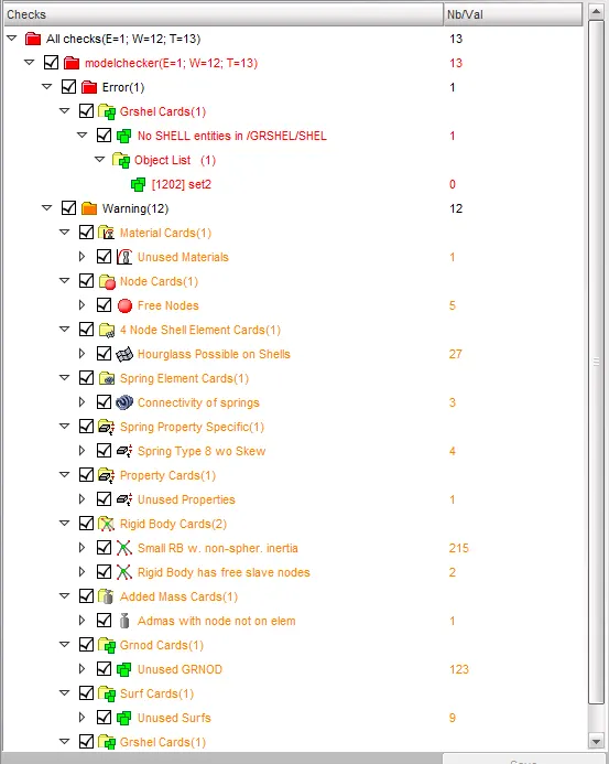
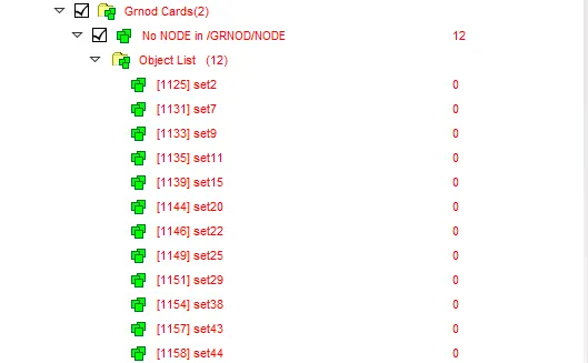
It analyses the model and displays the errors.

The errors I faced were only because of the empty set creation during the creation of the COG point and therefore, those empty sets can be deleted. Once the sets are deleted, the model can be exported again and it is imported into the HyperMesh and the simulation is run through it. The simulation will then run smoothly without showing any errors. If there is an error stating Error: 54, Go to the Cards tab in the Model Browser and delete the Unsupported cards entity and run the file for simulation. The simulation will be done smoothly within the given amount of time.

The Unsupported cards are created directly as the file is exported using the HyperCrash and thus, the solver has many other cards that are not used in Hypermesh and therefore creating new cards. When the file is opened again in the Hyper Mesh the file runs clearly but the cards which were created during the Hyper Crash are made into a single card as the unsupported cards and placed as an entity. The card can be deleted to make the simulation easy for the HyperMesh software.

(Note: The cards created in the Hyper Crash doesn't affect the model. It uses the required tools for it to run the model in the hyperCrash which is not used in the HyperMesh).

Results:

The Output file shows us the Error percentage and the number of steps for the given simulation. These are noted as follows.

Number of Cycles	80001
Total Run Time	7769.07 s
Energy Error Percent	-1.2%
Mass Error Percent	0.02999 %

The Simulation is completed successfully.

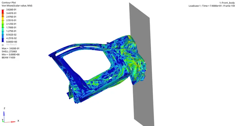
The Plotting of graphs is achieved successfully.

Energy Plots:

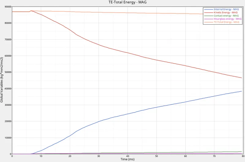
The energy plots are created between hourglass energy, Total Energy, Kinetic Energy, Internal Energy, and Contact energy versus Time.

Section Plots:

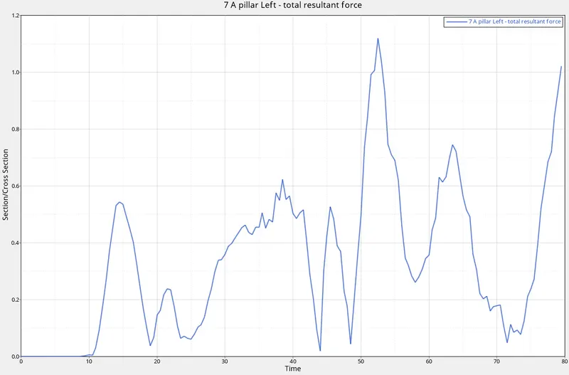
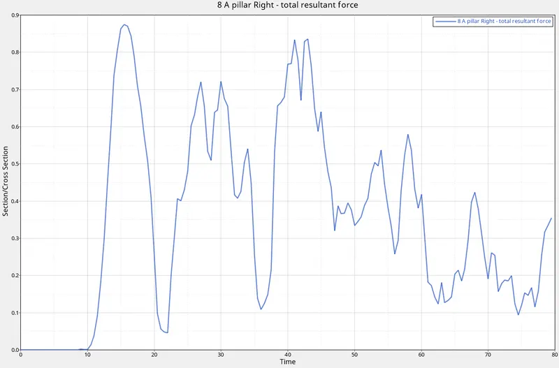
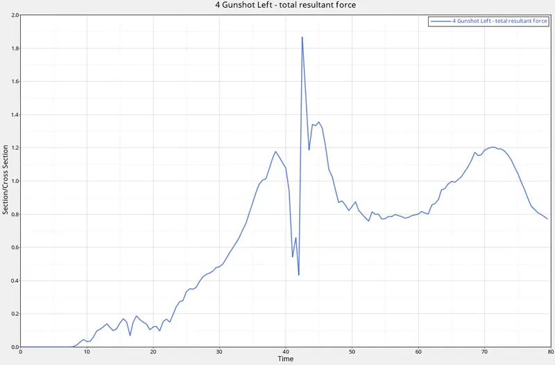
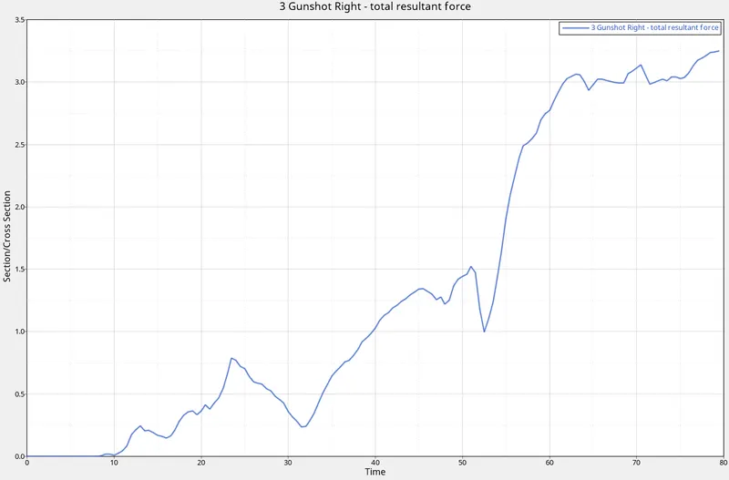
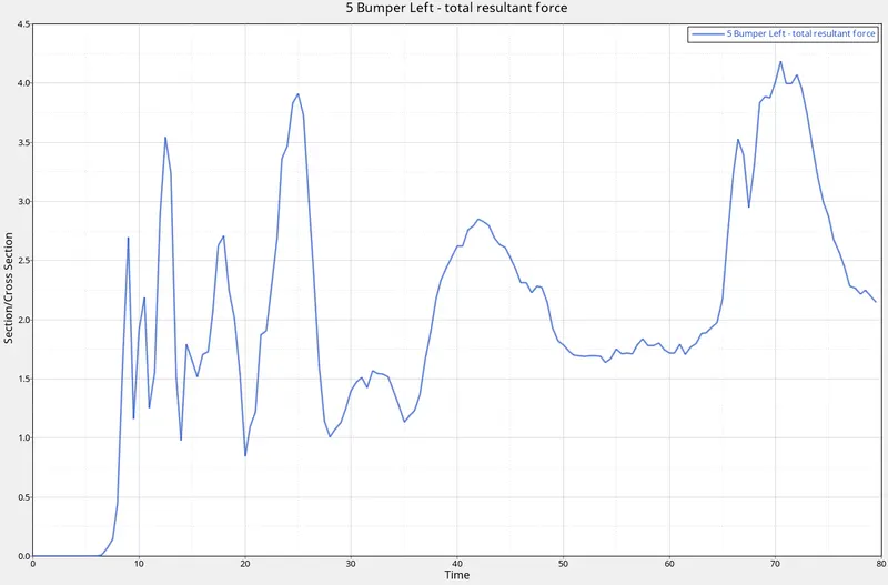
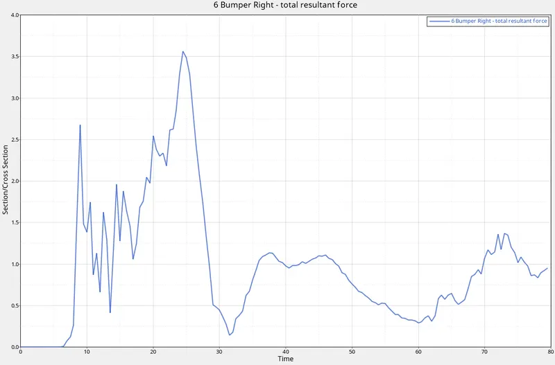
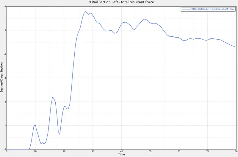
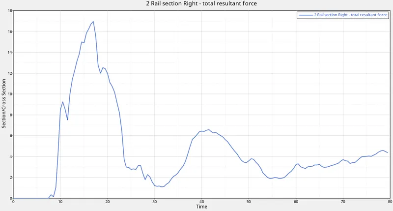
The plots for the cross-sections have different displacement values as the different components have different stresses acting upon them while performing a crash analysis.

The Graphs shown are the Force vs Time. They change to the force and load acting on it.

A-Pillar:

Shotgun:

Bumper:

Rail Section:

Observations:

It is observed that during the animation the deformation majorly takes place in the frontal area and the stress is passed to all the other components evenly by disrupting the shape of the frontal section but we can observe that the impact of the crash is taking only at the frontal region trying to save the driver seat area and the passenger seat but the impact is more and therefore it can injure the driver and passenger.

For the cross-sections of the parts, the Curve hits a peak value and the forces decrease after attaining the peak Force. The Cross-section creates a Force- time Graph and shows how the force is acting on the section at the particular time is known.

The Energy graph shows that the Hourglass and the Contact energy have a value near to zero. Total energy shows the summation of Internal energy and Kinetic energy. The decrease in the internal energy and the increase in kinetic energy leads to an almost straight line of the total energy.

For the Accelerations graph, the acceleration fluctuates drastically during the crash. Before the Crash, the acceleration will be maintained constant.

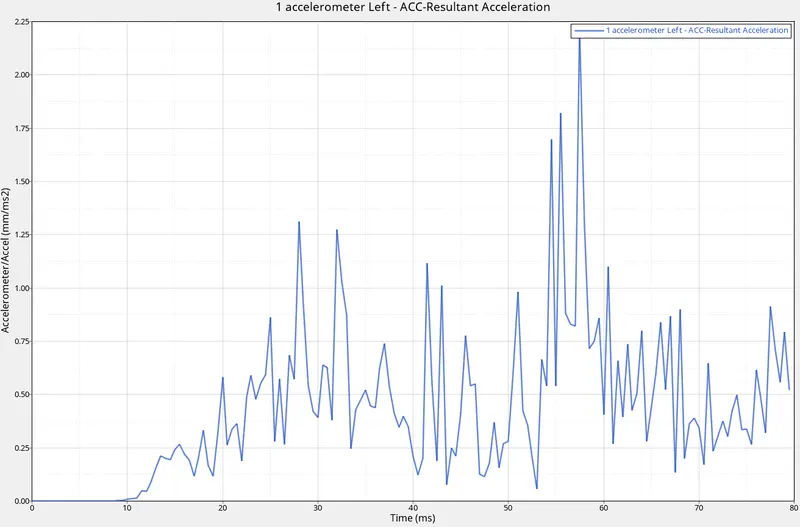
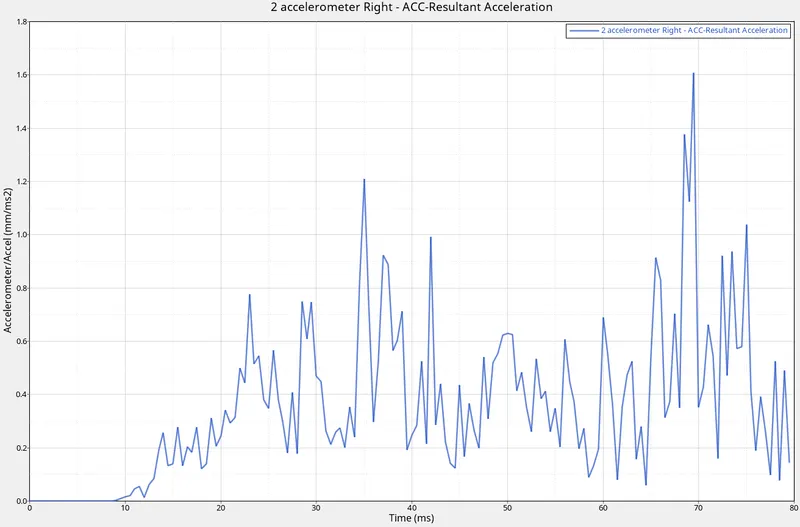
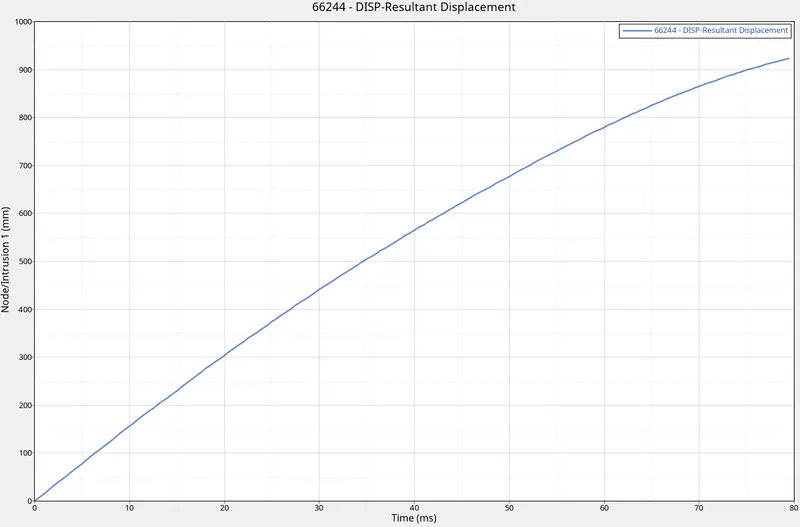
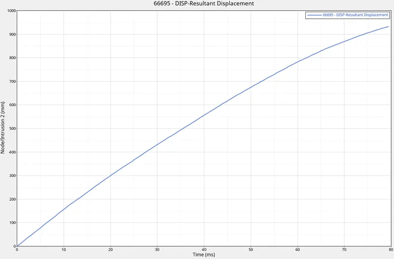
For the intrusions, the displacement curve is linearly increasing as the initial distance is noted as around 800mm but after the crash analysis, it is noted that the distance from the initial skew and final skew distance is around 900mm at the time 80ms.

Approximation is done considering both the cases.

Terms used:

Centre of Gravity:

The center of gravity (COG) of an object is the point at which weight is evenly dispersed and all the sides are in balance. A center of gravity can change as the mass changes but in many other cases, it's a fixed location.

Accelerometer:

An accelerometer is a device used to measure the acceleration (It is the rate of change of velocity) of a body. The accelerometer is typically used for linear type of acceleration based on vibration.

Type 7:

The general purpose of the TYPE 7 interface is that it can simulate all types of impact between a set of nodes and a master surface. Automatic node to surface contact gap can be constant or variable. The main advantage of this type of interface is that the stiffness is not constant and increases with the penetration preventing the node from going through the shell mid surface.

Rigid Wall:

The Rigid wall is a virtual wall created to perform the crash analysis on the body. The Rigid wall has no certain shapes or dimensions. It can be made as flexible as possible and It can sustain the load and thus, helping out to get a crashworthiness analysis.

Penetrations:

Penetration as the name suggests, a node gets penetrates the element and causes it to fail during the simulation. The penetrations are to be removed to get a better result.

Intrusions:

An intrusion generally means to get into one’s own property or territory. In HyperMesh Intrusions are checked to see if the component is withstanding crash making sure that the component doesn’t fail miserably.

Initial Velocity:

Initial velocity is the velocity of the object before the change in acceleration.

Learning Outcomes:

The Project covered all the basics of the topics learned during the course. The main outcomes learned are as follows

• Learned how to create an Initial Velocity, accelerometer, and Intrusions and how to call it.
• Learned to create cross-sections and to call it.
• Learned the topics of the interfaces and values that are recommended for the project.