Assignment 5-RADIOSS Interfaces & Study of Effect of Notches Challenge

OBJECTIVE:

1. Create the mesh for bumper assembly, mesh size should be 6mm.
2. Run the Crash tube model with 6 different cases as given below and compare.

• Run the crash tube model as it is.
• Change the Inacti=6 and run.
• Create the type 11 contact and run.
• Remove both notches and remove boundary condition on rigid body node then run.
• Create a new notch in the middle, select the whole section and run.
• Create a new notch with nodes only from opposing 2 faces and run.

1. MESH THE GIVEN BUMPER MODEL

PROCEDURE:

• Import file to hyper Mesh
• Delete solid surfaces
• Geometry clean-up
• Toggling lines
• Assign quality criteria
• Meshing
• Check for free edges

Procedure:

Model 1:

Meshing the given model(Bumper):-

• Initially, the user profile should be selected. As this model is to be only meshed. And hence no analysis is required, Radioss is selected is as a user profile
• Then the model should be imported into the HyperWorks software. After importing the geometry,

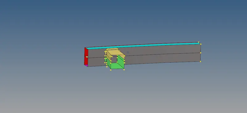
• The next step is to view the component by a topo. After switching it to the topo, the geometry in the graphical display

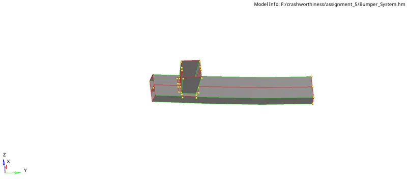
Geometry clean up:-

• The next step is to clean up the geometry. In the given bumper model, there are some surfaces which are intersecting with each other. So, this can be overcome by using the surface edit panel, trim with surfaces option

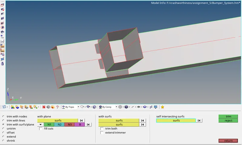
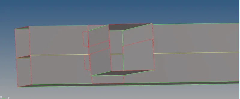
• So, here we have to toggle the free lines to get a shared edge
• Go to Quick edit >> Toggle >> Select line toggle
• If we want to Toggle a particular line:
• Toggle Edge > Right Click on the line

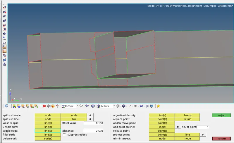
• After geometry clean up, the given bumper mode

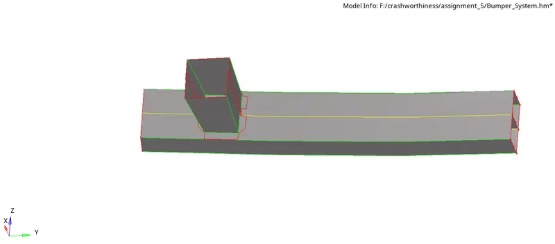
Meshing:-

• Before meshing, the parameters are element size is 6mm in the auto mesh panel should be selected. And then by selecting the surfaces by clicking on mesh, the mesh will be generated.

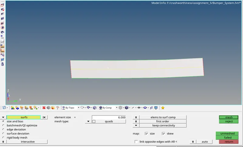
• After meshing, one surface of the mesh

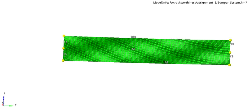
• After meshing the entire component, it appears as

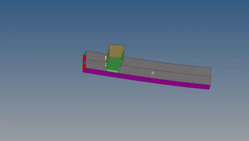
CHECK FOR FREE EDGES:

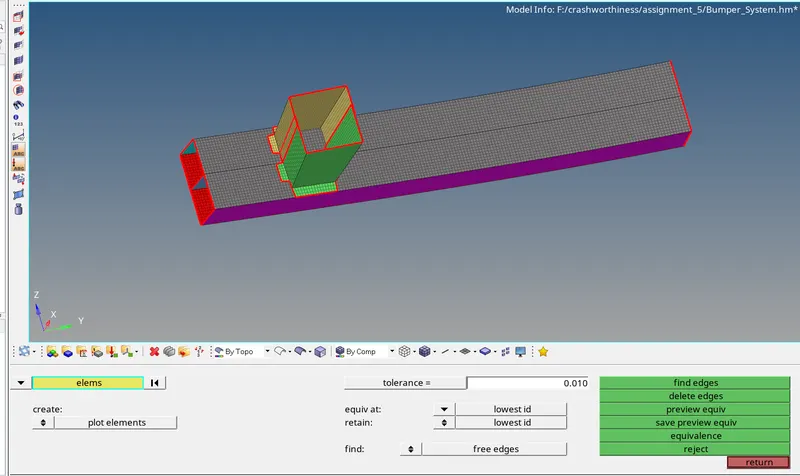
• we have to check for free edges (red lines) in the component.
• Edges Tool will help us find this error:
• Tool >> Edges [Shift + F3] >> Elem's >> Select by box selection >> Find edges
• If free edges are present, connectivity won't be established between the surfaces.
• As a result, when force is applied on any surface it won't be distributed to the neighboring surface due to a connectivity issue.

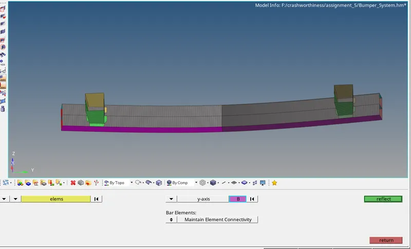
• After checking quality for the length and connectivity, the model can be reflected to represent the complete bumper as shown below.

Model 2:(Performing various cases on the given tube model):-

Case 1:(Running the model as it is by defining the TH for interfaces):-

• The next model is to analyze. So, the user profile chosen is "Radioss"

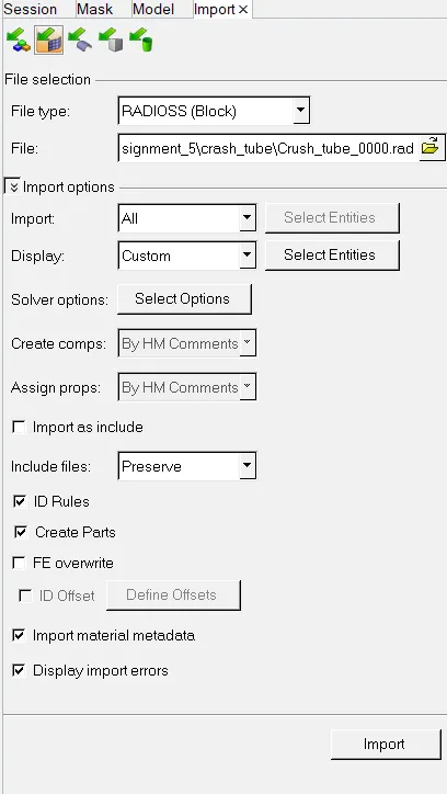
• Then the starter rad(0000.rad) file should be imported, from the import solver deck option in the menu bar,

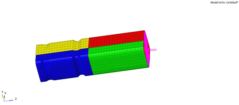
• After importing the file, the given model

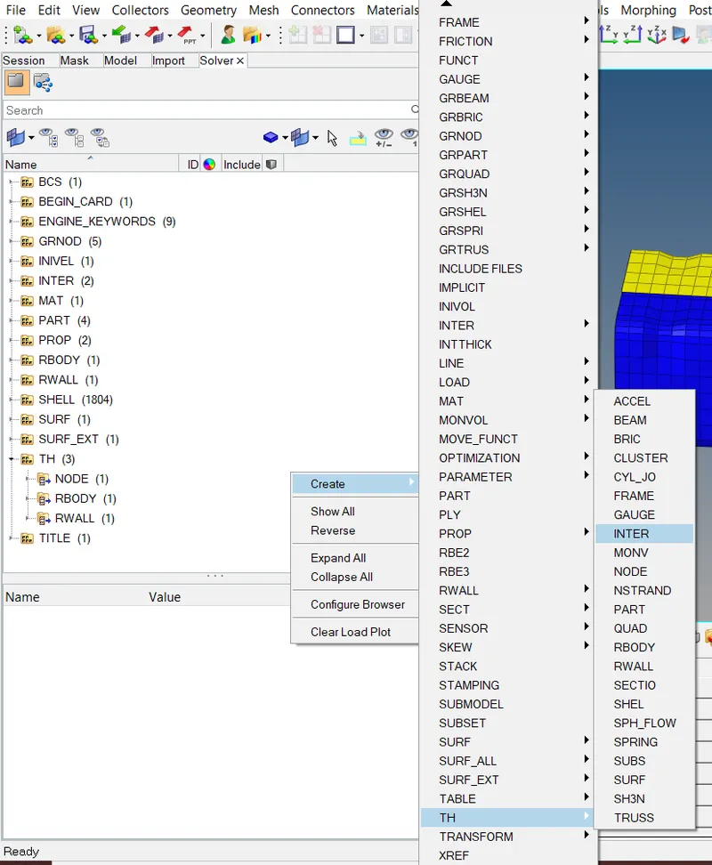
• As mentioned in the question, the output should be requested for interfaces or contact forces. So, the interfaces should be added to the TH. So, the TH is created for the interfaces

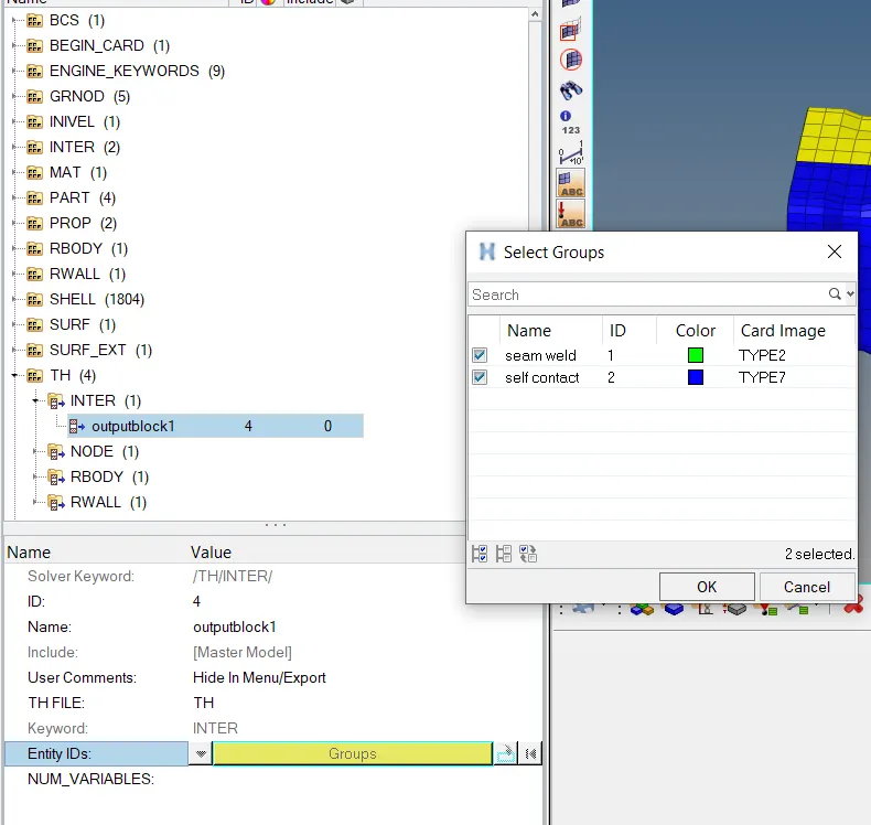
• After assigning the TH for an interface,Then the already created interfaces(represented in the form of groups) are assigned to the created TH,

• Then the simulation is to be run. The process of running the simulation is: Analysis panel---> Radioss

• Then the file should be saved in any location, Where all the animation files, time history files will be stored. And the "-nt 4" option is used to assign the task for the 4 cores in the CPU.

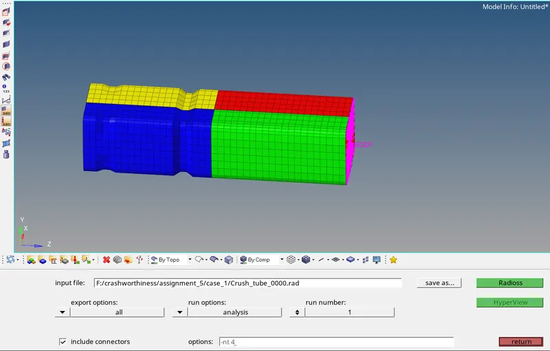
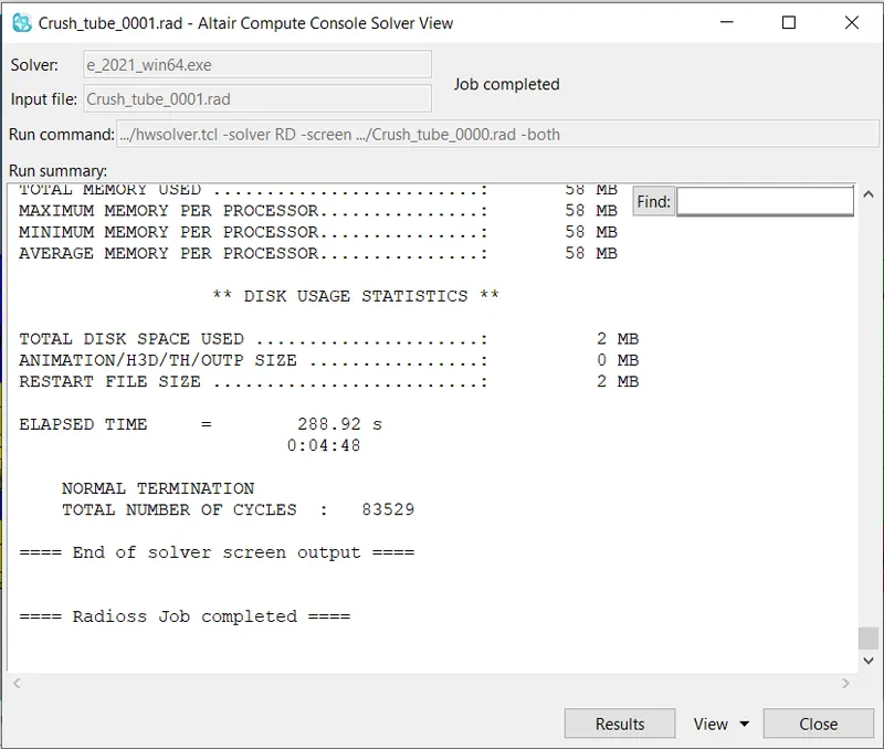
• Then by clicking on "Radioss", the simulation will be run. After some time, if the simulation is done properly and completed, it shows a pop-up. This indicates that the job is completed.

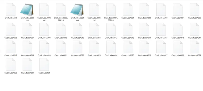
• The created animation files in the specified location

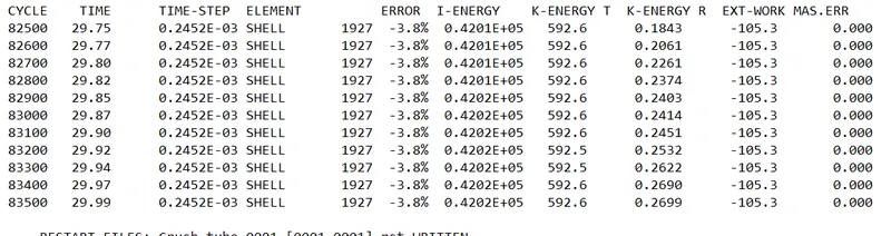
• Then the 0001.out file is opened, to view the obtained results in the form of values. The obtained results for the last cycle

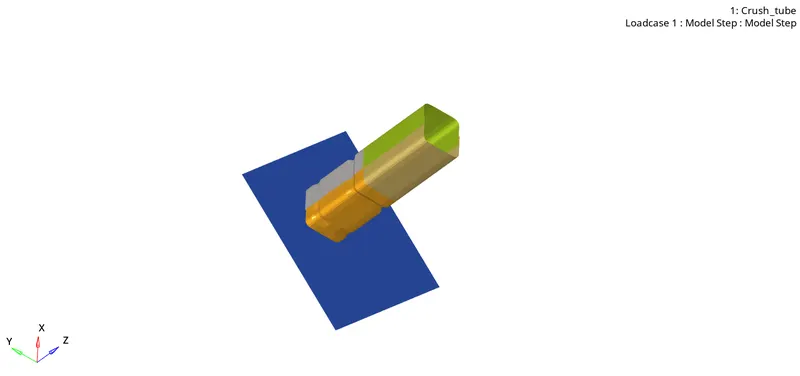
• Then the next step is to simulate the model with respect to the obtained files. For doing that, the h3d file(a combination of all animation files) is imported to another window. After importing the h3d file, the given crash tube model with the rigid wall appears in the graphical display

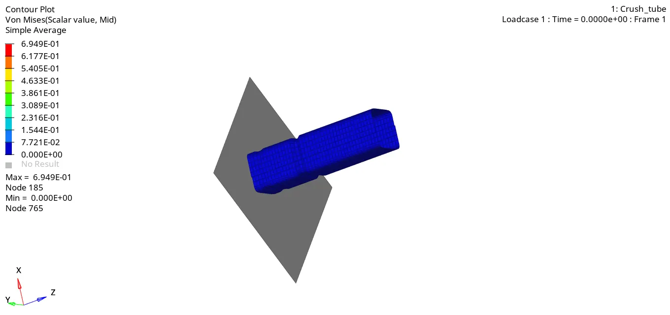
• Then the contour panel is opened and the parameters such as result type, selecting the components & averaging method are selected. Then it is applied. The obtained simulation in terms of von-mises appears as shown in the below animation.

Post-processing:

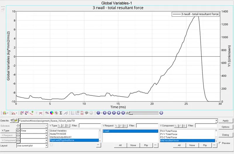
• The next step is to do the post-processing(i.e., obtaining the graphs with the help of obtained results). For doing that, the T01 file should be imported in the other window. After importing the parameters should be selected to obtain the graphs. Initially, the rigid wall force graph is obtained. So, the parameters should be selected
• The obtained rigid wall force graph. It goes on increasing. Because the forces within the elements start increasing at the beginning when the velocity is given. And when the entire tube collides with the rigid wall, the rigid wall forces reach the peak value. Due to this the contact energy increases, which results in the increase in rigid wall forces.

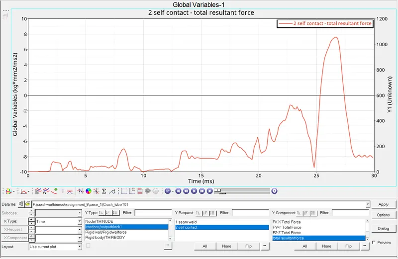
• The next graph to be obtained is the contact forces graph. Some parameters should be selected as interference. To obtain the graph.
• The obtained contact force graph. Initially, there will be no contact forces at the beginning. So, the curve starts from origin. And there will be some fluctuations in the curve in the middle. Due to fluctuation of contacts within the elements. And then it reaches the peak value, when the entire model undergoes collision, there will be more contact within the elements & even with a rigid wall.

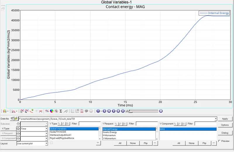
• Then the final graph to be obtained is the internal energy graph. The parameters to be selected in order to obtain the graph
• The obtained internal energy graph. The internal energy increases to the peak value at the end of the collision. And becomes constant.

Case 2:(Changing the inacti value to 6):-

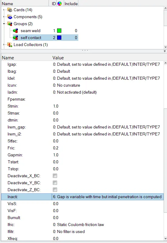
• In this case, In the interfaces card, the inacti value is changed to 6. Then, the simulation is run. With this, the gap will be scaled further in between the slave & master.

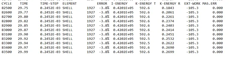
• After running the simulation, the obtained 0001.out file is opened. To view the obtained results in the form of values. The obtained results for the last cycle

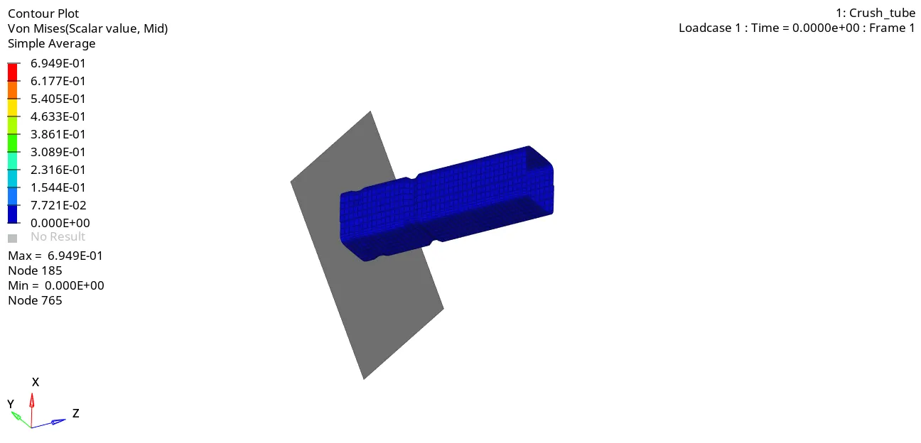
• Then the obtained simulation from the h3d file in terms of von-mises stress appears as shown in the below animation.

Post-processing:

• Then the To1 file is opened in another window. In order to view the results in terms of graphs. The obtained rigid wall force graph. It goes on increasing. Because the forces within the elements start increasing at the beginning when the velocity is given. And when the entire tube collides with the rigid wall, the rigid wall forces reach the peak value. Due to this the contact energy increases, which results in the increase in rigid wall forces. It will be somewhat similar to case 1.

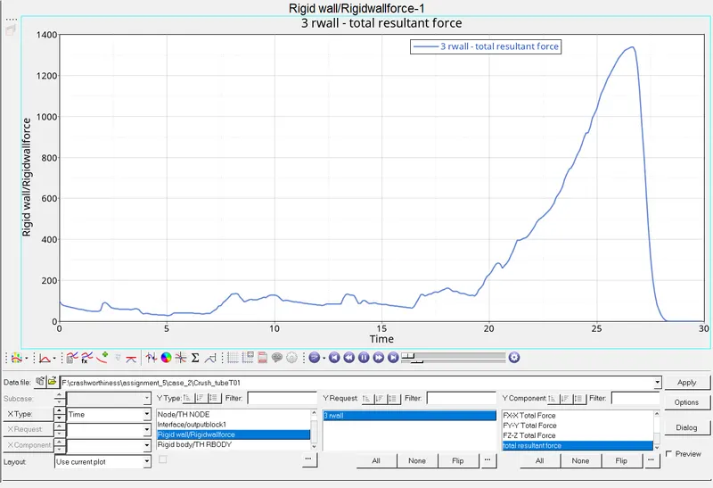
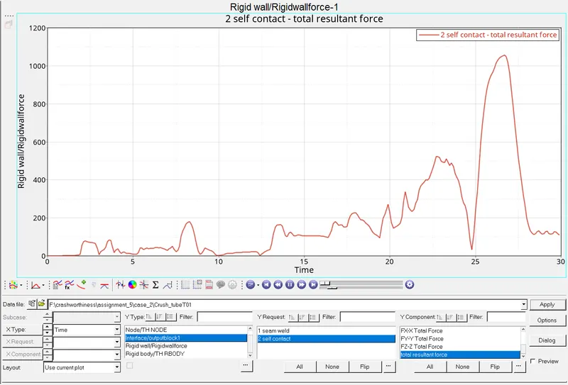
• Then the graph to be obtained is contact forces. The obtained contact force graph. Initially, there will be no contact forces at the beginning. So, the curve starts from origin. And there will be some fluctuations in the curve in the middle. Due to fluctuation of contacts within the elements. And then it reaches the peak value, when the entire model undergoes collision, there will be more contact within the elements & even with a rigid wall. It will also be somewhat similar as in case 1. Because there are no initial penetrations.

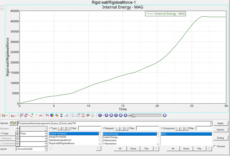
• Then the internal graph is obtained. The obtained internal energy graph. The internal energy increases to the peak value at the end of the collision. And becomes constant. As there is no change in the above graphs, there is a change in the internal energy graph also.

Case 3:(Creating the type 11 contact):-

• In this case, the new contact named "Type 11". In this contact, some parameters are to be entered. In order to get, better results.

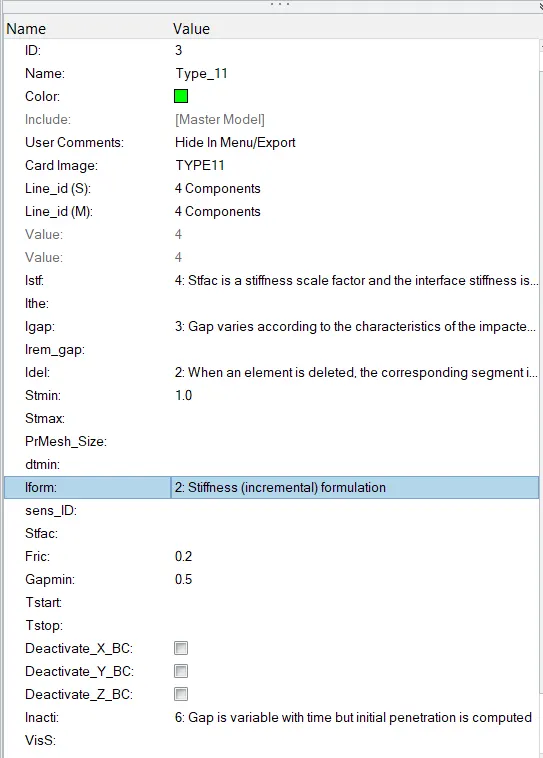
• While defining the slaves & master, ensure that all elements should be as a slave & as well as master,

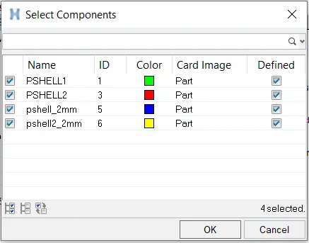
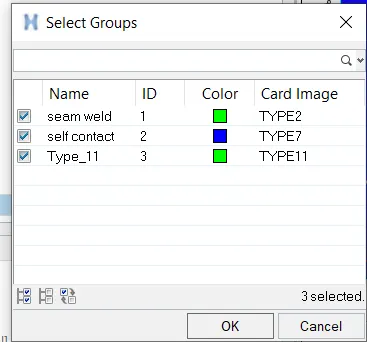
• After creating the contact, then for obtaining the output a TH is requested for that contact. While defining the TH for that contact, the interfaces should be entered

• After running the simulation, the obtained 0001.out file is opened. To view the obtained results in the form of values. The obtained results for the last cycle

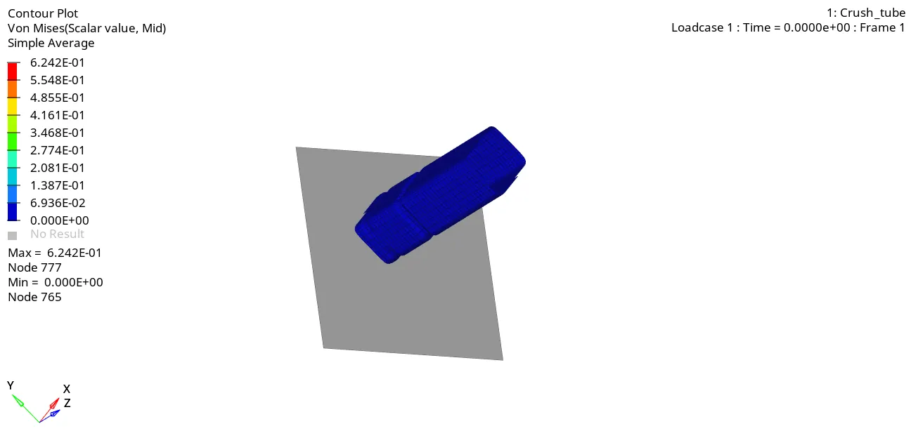
• The next step is to run the simulation. After running the simulation, the obtained simulation from the h3d file in terms of von-mises stress appears as shown in the below animation.

Post-processing:

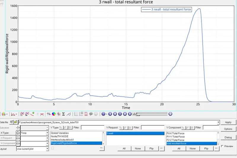
• Then the post-processing is done. The obtained rigid wall force. From that graph, The thing noticed is the rigid wall force value is increased (Within the range 1400-1600) when compared to the previous cases. The reason is, Type 11 contact is also defined along with the pre-defined type 7 contact. So, the contact forces with respect to the edge-to-edge contacts are also seen.

• The next graph obtained is, contact forces with respect to type 7 contact. The obtained contact forces graph for type 7 contact. The contact forces will be constant and reach the peak value when all of a sudden the nodes come in contact with the master elements within the tube model. And the graph falls back when the model attains reaction against the rigid wall.

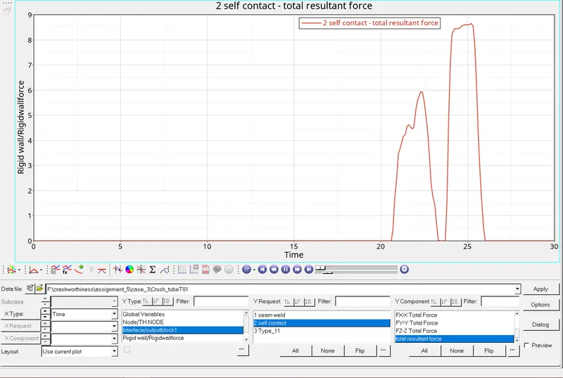
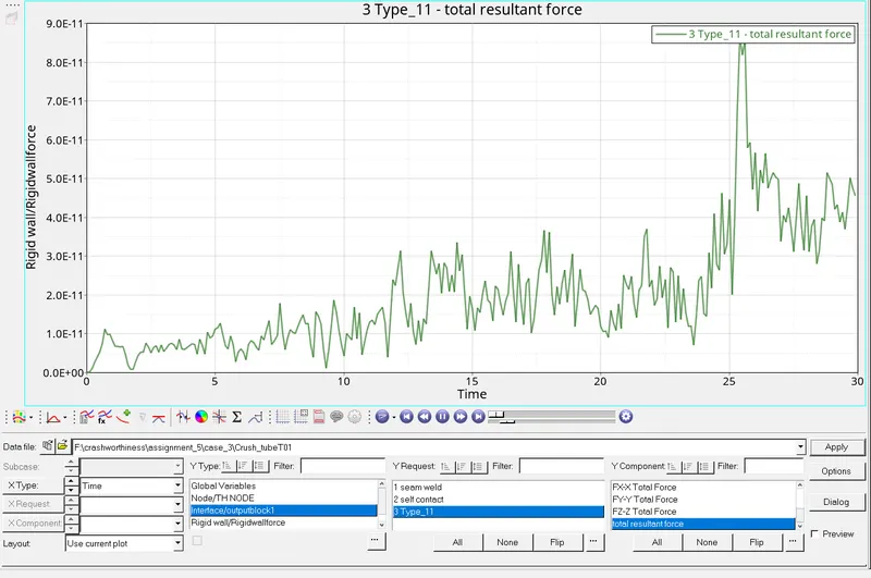
• Then a graph is obtained for the type 11 contact. The obtained graph for type 11 contact. This graph depicts the edge-to-edge contact. There will be fluctuations, as the edges of the elements come into contact gradually. ANd reaches a peak value, after the entire collision. And decreases thereby due to the little expansion of the model after hitting the rigid wall.

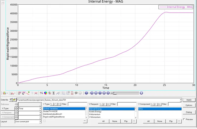
• Then a graph is obtained for the internal energy. There will be no change in the kinetic energy.

Case 4:(Running the given model by removing the notches & boundary condition on the rigid body node):-

• In this case, the notches are removed & the pre-defined boundary conditions are also removed. For removing the notches, the option used is "Align node". The keyboard shortcut for that is "Shift+F8".

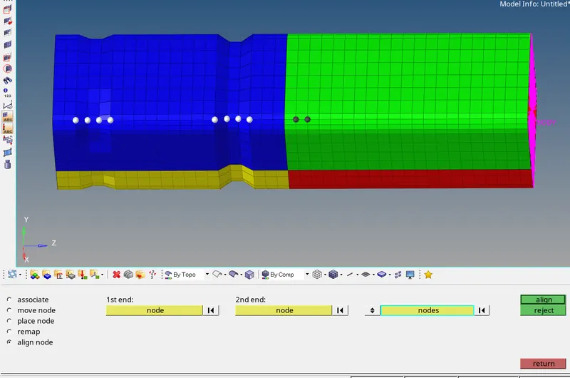
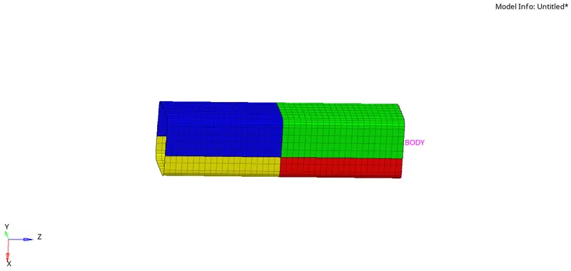
• After removing the notches,

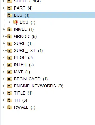
• The next step is to remove the boundary condition on the rigid body node. Which is present in the tab bar in the solver browser

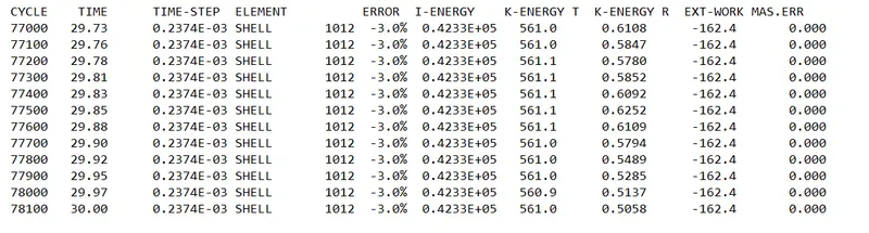
• Then the obtained 0001.out file is opened. To view the obtained results in the form of values. The obtained results for the last cycle

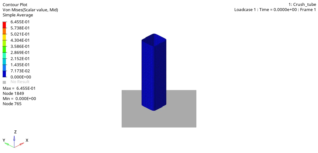
• Then the simulation is run. After running the simulation, the obtained h3d file is imported into another window. To view the simulation. The obtained simulation appears as shown in the below animation.

Post-processing:

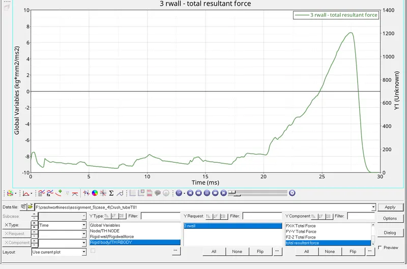
• The next step is to go for post-processing. The obtained rigid wall graph. In this case, the rigid wall force is reduced when compared to the previous cases. The maximum values lie in the range of 1000-1200 N. This is due to the removal of notches. As the notches are removed, there will be a change in element shape at the notches, which results in the reduction of rigid wall forces.

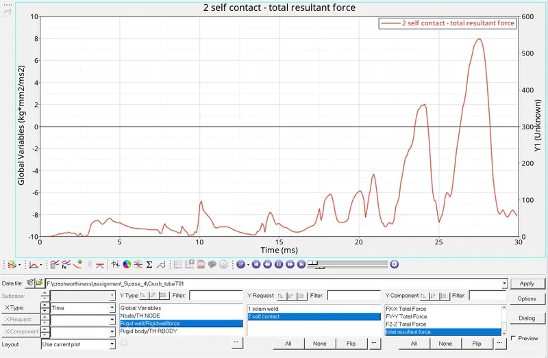
• Then the obtained contact force graph. There is a reduction in the contact forces. Because the notches & boundary conditions are removed. So, the energy will be observed by the elements will be faster when compared to the previous cases with the notches.

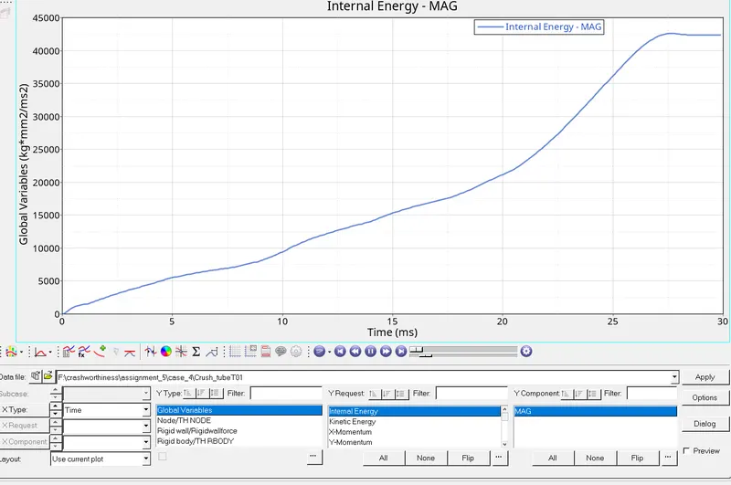
• The obtained internal energy graph. There will be no change in the internal energy when compared to the other cases.

Case 5:(Running the simulation by creating the notch at the middle):-

• In this case, a notch is created at the middle of the tube. This is done by using the "Translate" option. The magnitude is selected as 2.5 mm to translate. Because it is calculated by using the Pythagoras theorem in the model for the previous case. And the model with case 4 is chosen to open here. Because it doesn't have notches.

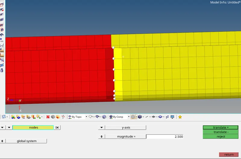
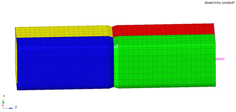
• After translation of nodes at the middle

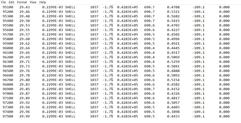
• Then the obtained 0001.out file is opened. To view the obtained results in the form of values. The obtained results for the last cycle

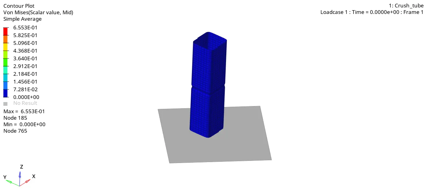
• Then the simulation is run. After running the simulation, the obtained h3d file is imported into another window. To view the simulation. The obtained simulation appears as shown in the below animation.

Contact energy:

• Contact Energy is the energy acting opposite to the system to prevent the penetration acting on the system. When the force is applied to the body, the crush tube starts to deform but the penetration happening is low in the initial stage. The contact energy will below.
• Once the deformation is maximum, the elements will be forced to penetrate but the opposite force which is contact energy will also increase which helps in the prevention of penetration. Once the deformation ends, the contact energy will become zero and will stay constant thereafter.
• In this case, the contact energy incurred is more when compared to case 1 and case 2. This is due to only one notch at the center which increases the rate of deformation, which intern increases the rate of penetration.

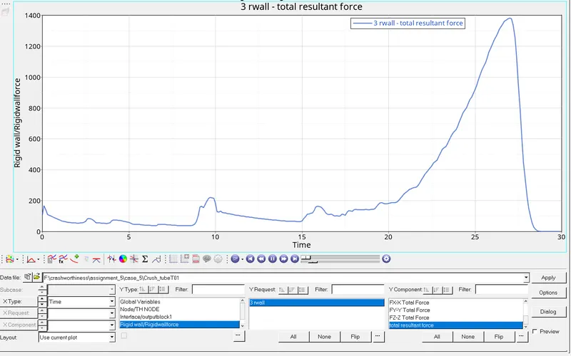
• The obtained graph for internal energy. There will be a change in the internal energy. Because, As there is a notch only at the middle. The elements will be impacted without any deviation, as of in the previous cases in which the notch is present at the beginning. There will be a drop in the internal energy at the middle as shown in fig. Due to the model moves back after hitting the rigid wall. And there will be a rise again. Because the model again hits with the elements after notch.

Case 6:(Running the simulation by Creating a new notch with nodes only from opposing 2 faces):-

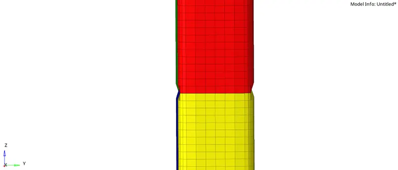
• In this case, the new notch is created in the middle again. But only at the two opposite faces.

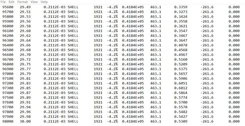
• Then the obtained 0001.out file is opened. To view the obtained results in the form of values. The obtained results for the last cycle

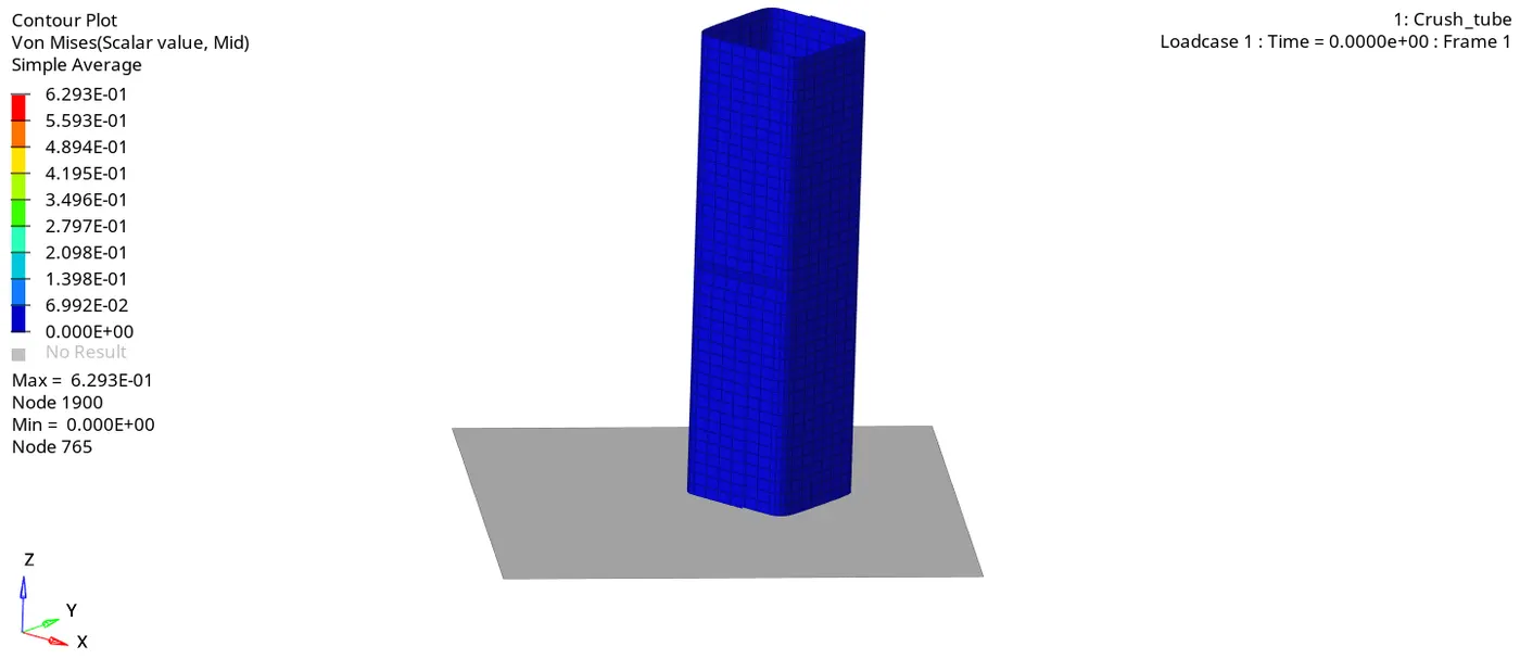
• Then the simulation is run. After running the simulation, the obtained h3d file is imported into another window. To view the simulation. The obtained simulation appears as shown in the below animation.

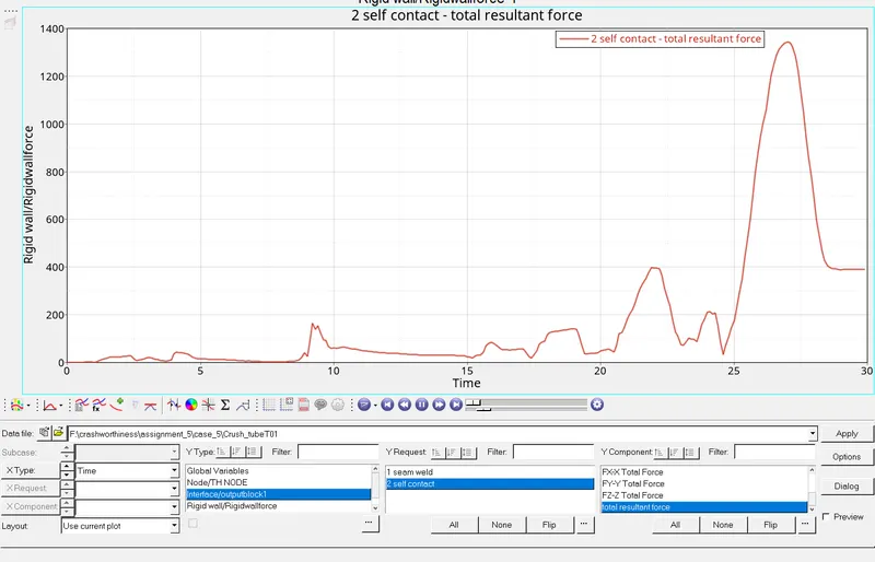
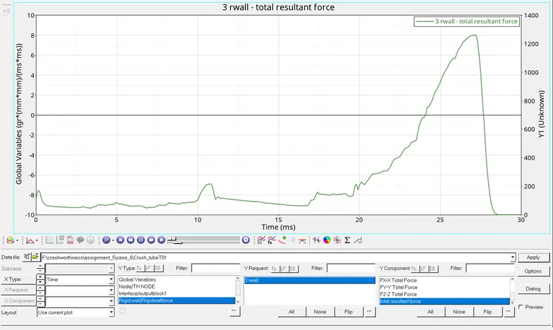
• The obtained rigid wall force graph. There will be a rise in rigid wall force when the entire collision takes place. The area with the notch will be experiencing more stress.

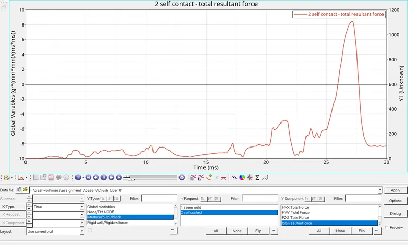
• The obtained interface force. The contact interface rises at the end of the collision.

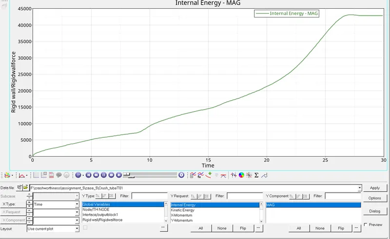
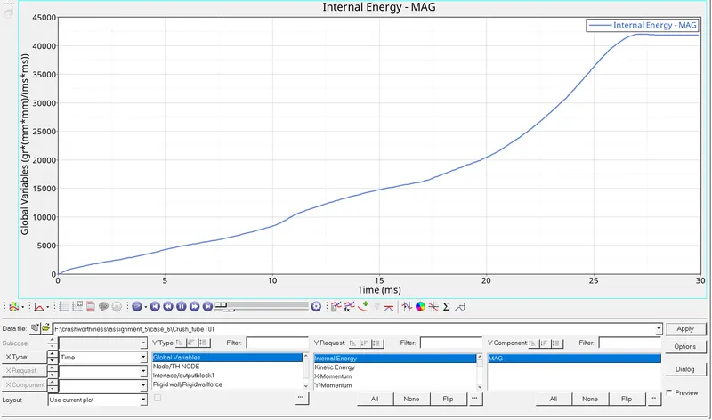
• The obtained internal energy graph for this case. There is a change in internal energy due to the notch. Because the notch area will experience high stress & deflect stress.

Comparison of above cases:-

Basis for comparison	Case 1	Case 2	Case 3	Case 4	Case 5	Case 6
Enenrgy error(%)	-3.8%	-3.8%	-7.8%	-3.0%	-1.7%	-4.2%
Mass error(%)	0	0	0	0	0	0
Max Von-mises stress	6.949E-01	6.949E-01	6.413E-01	6.518E-01	5.997E-01	6.312E-01
Internal energy(KJ)	0.4202E+05	0.4202E+05	0.4036E+05	0.4233E+05	0.4283E+05	0.4184E+05
Kinetic energy(KJ)	592.6	592.6	575.0	561.0	690.5	463.1
External work	-105.2	-105.2	-123.7	-162.4	-109.1	-261.6
Notches	Notches will be there.	Notches will be there	Notches will be there	No notches	A notch at the middle of the model	Notches at the opposing faces in the middle.

Conclusion:

• Generated the mesh for the given bumper component with a mesh size of 6 mm.
• Changed the parameters for the given crash tube model as various cases.
• Finally, plotted the graphs with RWALL forces, contact forces, internal energy (Post-processing) & compared the results.

Learning outcomes:-

By doing this challenge, the following aspects can be learned:

• Observing the variation in results with respect to the change in notches.
• Observing the behavior of crashes by various cases.