To study the Interfaces used in HYPER-MESH for defining the contact between the element to perform the Analysis of Automotive Components

Aim -

To perform the impact analysis on the crush tube by impacting on the rigid wall in HYPER-MESH & RADIOS.

Objective -

Mesh the Bumper System of Automobile and Analyze the Crush Tube using different interface properties.

Abstract -

1] Mesh the Bumper System with a mesh size of 6mm and Seam weld the edges.

2] Analyze the Crush Tube by setting the interface contact for different Cases.

Part I - Mesh the Bumper System:

Step 1 - Open the model:

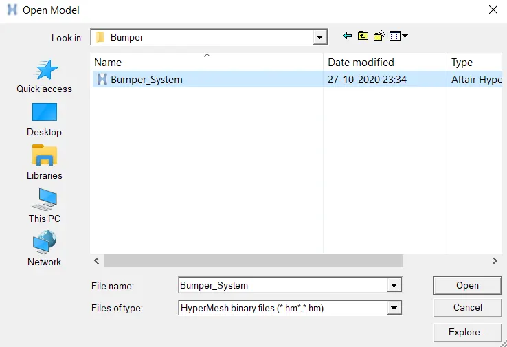
fig - Importing the model to Hypermesh

Step 2 - Check for the geometry errors:

After importing the geometry in the hypermesh first task is to check the geometry error. This error has to be identified manually over the component.

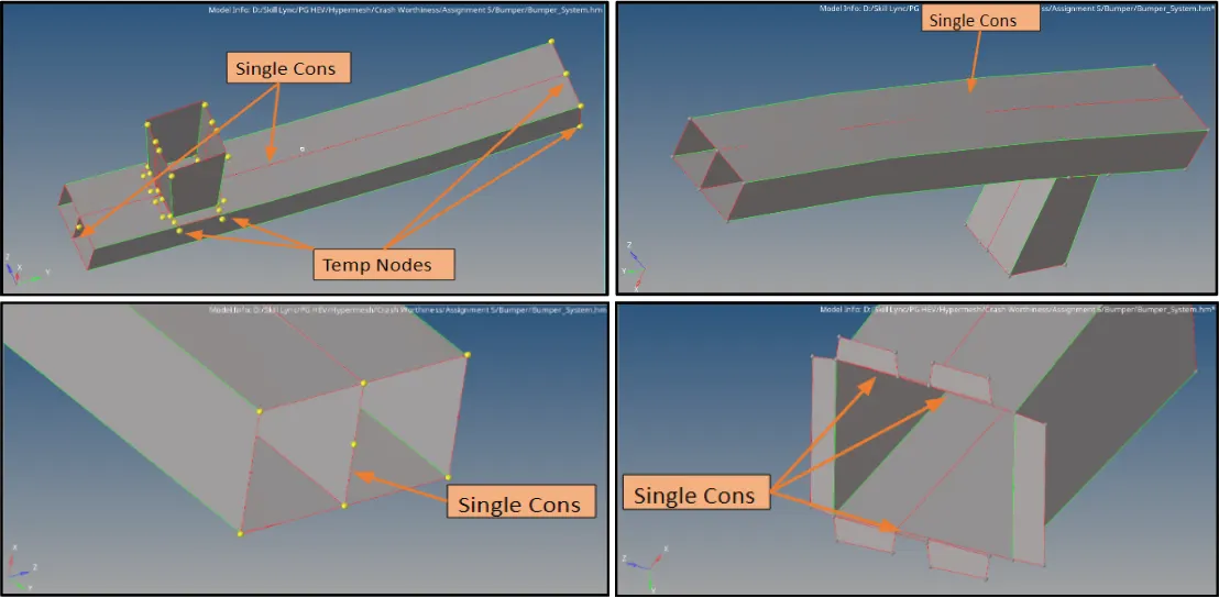
fig - Geometry Errors

After Geometry Cleanup

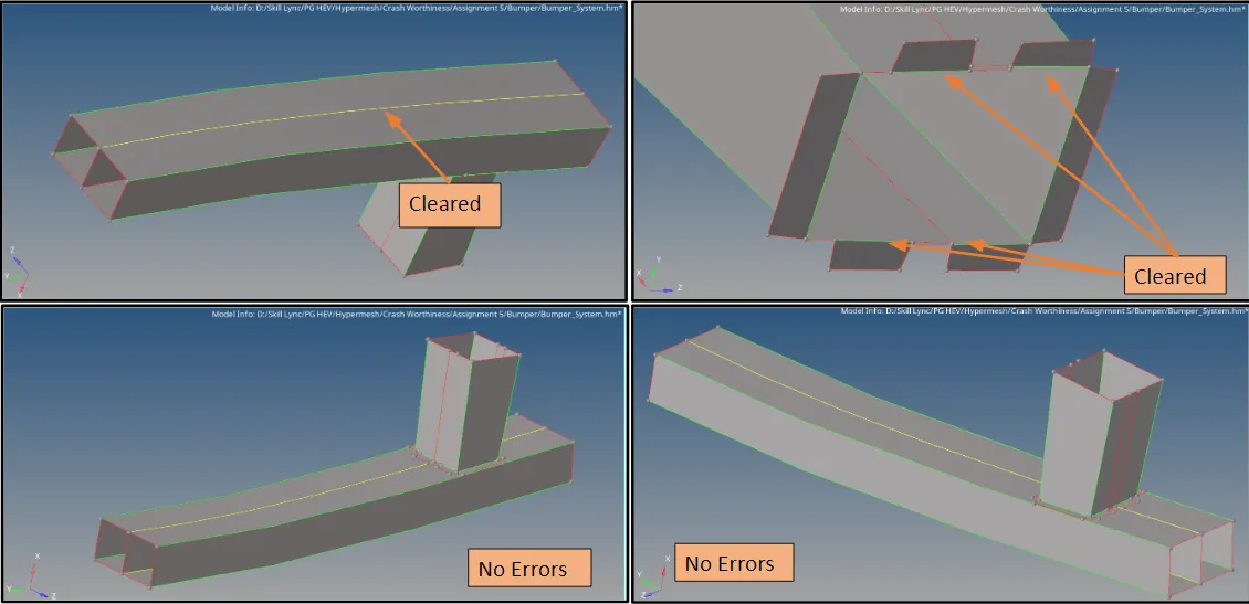
fig - Geometry Errors Free

Step 3 - Meshing the Geometry:

After cleaning the geometry the next step is to mesh the geometry. For meshing the geometry under 2D auto mesh tool is used with the element length of 6 mm.

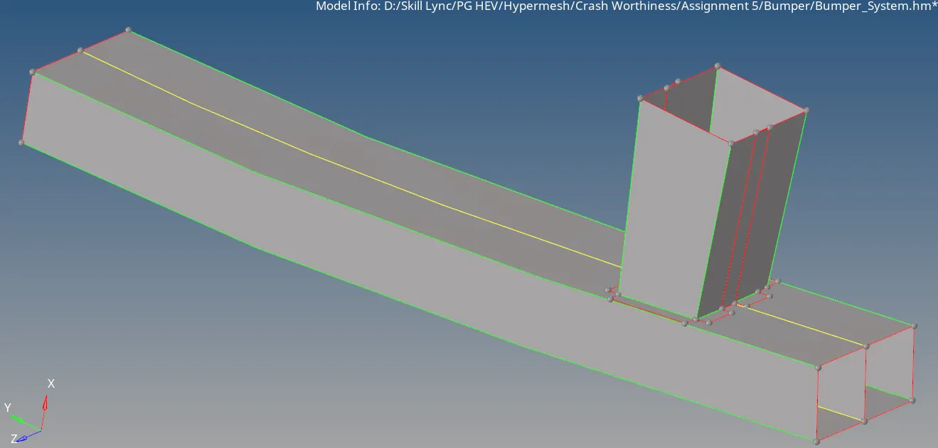
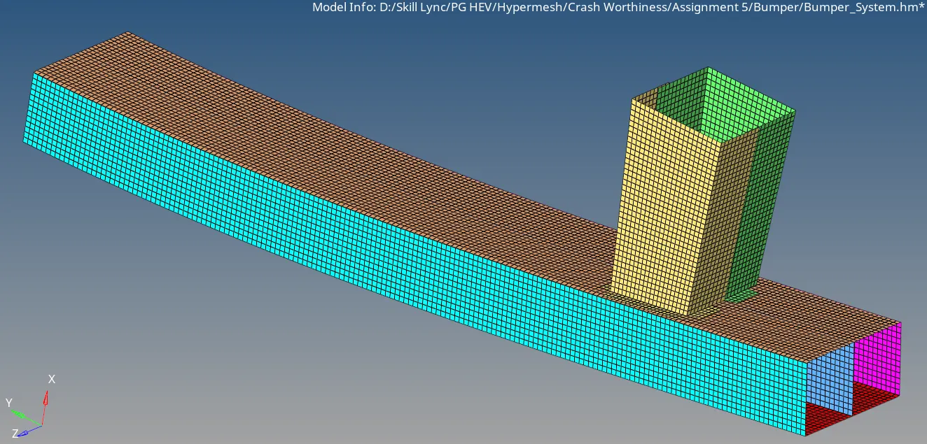
fig - Meshed Geometry

Step 4 - Connection (Seam Weld):

As we see that the crash box is not connected to Bumper Beam Rear so to connect that connections are deployed between both of them with a help of the Seam weld tool in the 1D Panel. The connection is deployed as shown below.

Process flow:

1D --- Connectors --- Seam --- Location (Select Nodes by Path) --- Spacing (6 mm) --- Tolerance (10) --- Type (Spring 2 Single Row) --- Select Component to be Weld --- Create

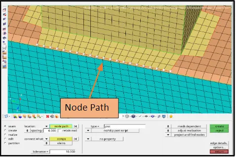
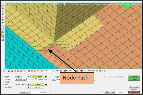
fig - Connection - Seam Weld

Step 4 - Reflect:

After deploying the connections between the components next step is to reflect the element to the opposite side in the y-axis. For this, under the tool panel, there is an option called to reflect. With the help of this tool, we can easily reflect the half geometry to the full one.

Process Flow:

Tool --- Reflect --- Select elements to reflect (As displayed) --- Duplicate the Elements --- Axis of Reflection & Bar Point --- Reflect

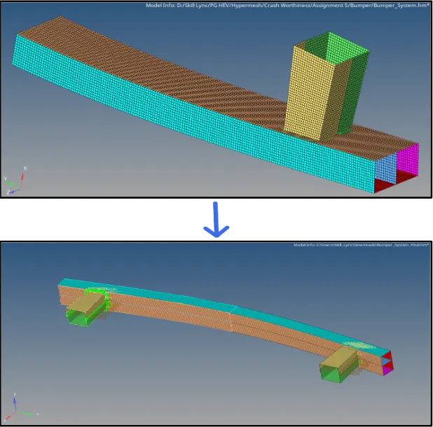
fig - Reflected Geometry

Part II - Crash Tube Analysis by examining the interface of the elements:

Before going to the model first we see what is Interface / Contact Modelling?

What does Interface mean?

The interface means how the elements behave with each other when they are in contact. The explicit analysis method efficiently solves complex dynamic contact problems (boundary condition nonlinearity). Accurate modeling of contact interfaces is essential to correctly capture contact interaction between bodies. RADIOSS has a large number of contact types suitable for many applications.

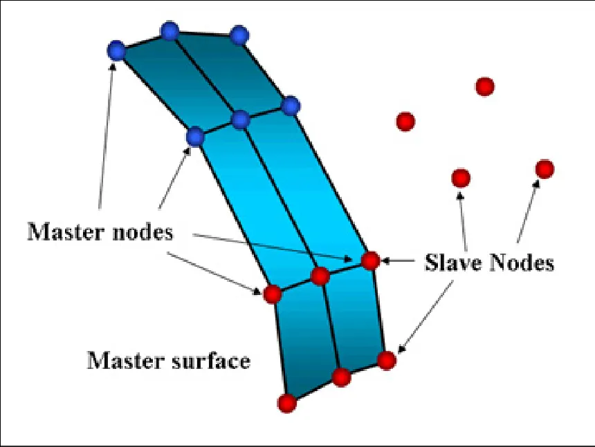
In RADIOSS an interface is created by defining the master segment and slave node-set. The master segment can be parts of components, elements, contact surface, node surface sets, and slave entities that can be parts of components and node sets. The contact algorithm will check every time step for potential penetration of a slave node through a master segment. If penetration is detected the contact is treated with either a Penalty or Lagrange multiplier method.

In this project we will learn about:

• TYPE7, variable stiffness, node to surface contact
• TYPE11, variable stiffness, edge to edge contact

The Penalty Method Used In Interfaces:

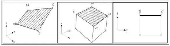
Interfaces using the penalty method are based on master/slave treatment. Contact can only occur between a set of slave nodes and a set of master segments. Master segments are defined depending on the type of element they lie on. If it is a 3-node or a 4-node shell, the segment is the surface of the element. If it is a solid element, the segment is defined as a face. Finally, if it is a 2D solid element (quad), the segment is aside.

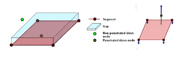
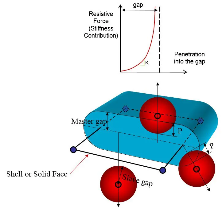
A gap distance is defined to determine whether or not a node is in contact with a segment. Spring elements that generate resistive forces as a function of penetration are created between the slave node and its projection. The spring stiffness is automatically computed according to the material and property of both the master segment and the slave node. The time step may be affected by the interface stiffness. During the penetration, as the spring is connected to the slave node, the spring stiffness must be added to the overall stiffness acting on the node (stiffness from all elements connected to this node). The nodal time step must be reduced to account for the spring stiffness. Contact ends when the penetrated node is completely pushed out of the gap. Therefore, the elastic spring and the reaction forces are removed. It is worthwhile to note that the contact interfaces with the penalty method are fully compatible will all kinematic conditions (for example, a rigid body, imposed velocity, etc.).

Lagrange Multiplier Method (/LAGMUL and /INTER/LAGMUL):

Contrary to the penalty method, the Lagrange Multiplier method is purely mathematical and does not require physical elements (springs) to model contact. A nonlinear system of equations is solved to account for contact conditions. Therefore, there is no time step collapse due to high interface stiffness, but it takes more CPU time to do one cycle as new equations need to be solved by a nonlinear solver. The method has the advantage to stop slave nodes at the contact surface (the contact condition is precisely satisfied); however, the friction cannot be computed.

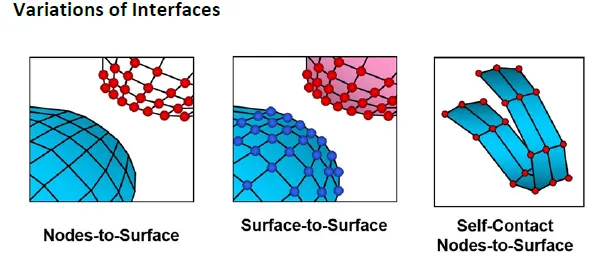
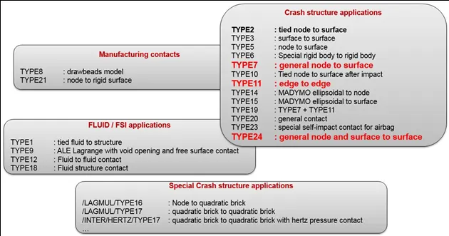
Types Of Interfaces Used In RADIOSS

Interface Type 7: Nodes to Surface Contact:

• Automatic node to surface contact interface using penalty method with variable stiffness
• A gap is defined around the master segment and the slave nodes
• The contact gap can be constant or variable
• Resistive forces are applied to keep slave nodes out of the contact gap
• Interface time step is computed to ensure stability

Interface type 7 is a general-purpose interface and can simulate all types of impact between a set of nodes and a master surface. Contrary to interface types 3 and 5, interface type 7 is non-oriented and slave nodes can belong to the master surface. Therefore, this interface can simulate auto-impact, especially buckling during a high-speed crash. Interface type 7 solves all problems and limitations encountered with interface types 3 and 5. The search for the closest segment is done via a direct search algorithm; therefore, there are no search limitations and all possible contacts are found. The energy jumps induced by a node impacting from the shell edges are removed by the use of a cylindrical gap around the edges.

Important Interface Parameters:

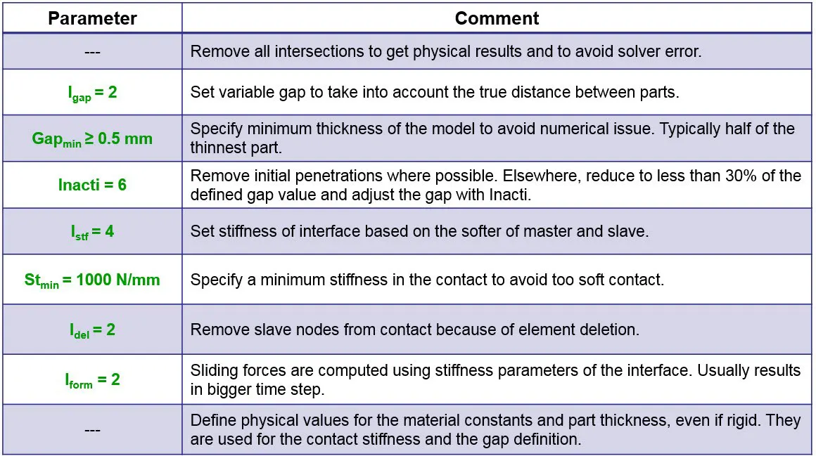
Igap - Determines how the size of the gap is calculated
Gapmin - Minimum gap for activation of the interface
Inacti - Action to take if initial penetrations exist
Istf - Affects how the stiffness of the interface is calculated
Iform - Friction formulation
Stmin - Minimum stiffness to use in the interface
Idel - Update For Deleted Elements Due To Failure

Interface Type 7: Recommendations For Crash Applications:

Non-Linear Type7 Advantages & Disadvantage:

Advantages

• Best used with shells to shells or solids to shells
• Physically correct representation
• High accuracy for describing self-contact and buckling

Disadvantages

• Requires more stringent modeling practices
• Does not tolerate intersections (slave node passing master segment)
• Time step may reduce due to increasing interface stiffness

Limitation Of Nodes-To-Surface Interface:

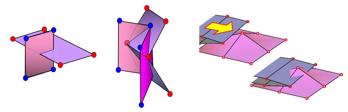
There are situations where the Type 7 node to surface interface will not detect the contact due to edges crossing each other at angles. Type 11 interface can be added to capture the physics correctly.

Interface Type 11: Edge to Edge Contact:

• This interface simulates the impact between edge to Edge or lines. A line can be a beam or truss element or a shell edge or spring elements. In association with interface TYPE7, interface TYPE11 solves the locking cases
• Defined by identifying master and slave lines (edges)
• Impacts occur between a master and a slave line. A slave line can impact one or more master lines. A line can belong to the master and the slave side. This allows self-impact.
• Works similar to Type 7 in terms of Penalty formulation, Gap definition, and Search method.
• Uses complicated mathematical algorithms; therefore, it is strongly advised to use it only when necessary. A huge interface TYPE11 can slow down the computation.

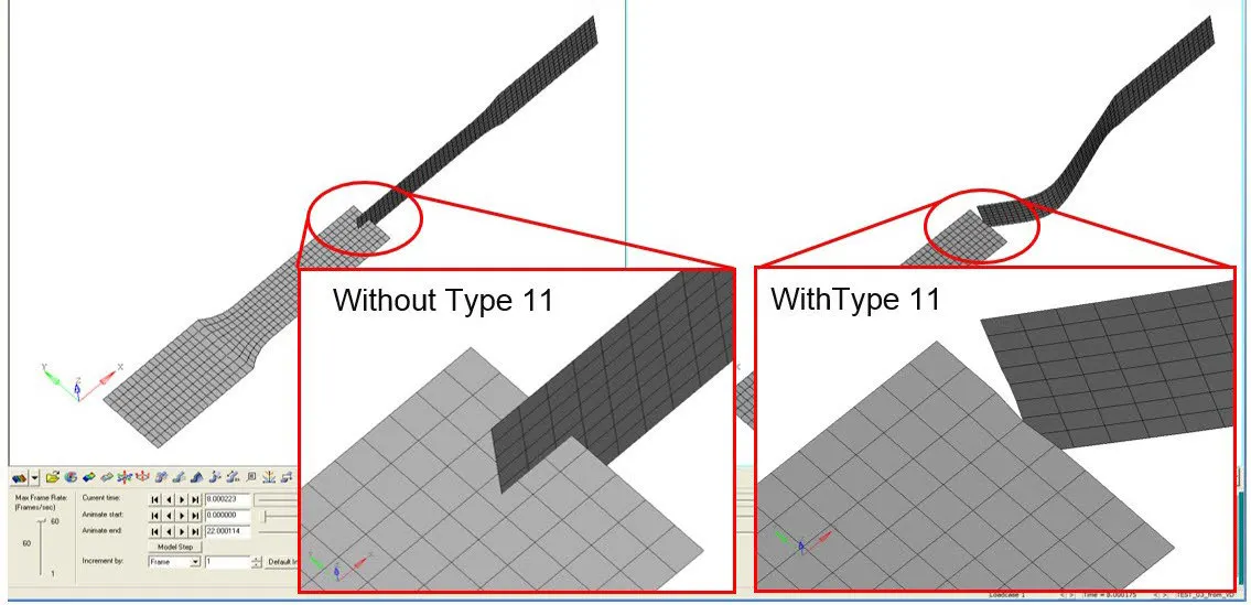
A General Remark About Master & Slave:

The coarser the mesh, the stiffer the structure will be provided the material and structural properties are the same. Hence, the Master has typically meshed coarser so that the Slave does not penetrate the master. That is why we choose a stiffer structure as master and compliant as a slave.

Case I - Run the crash tube model as it is

First Import the model from the folder where it is saved,

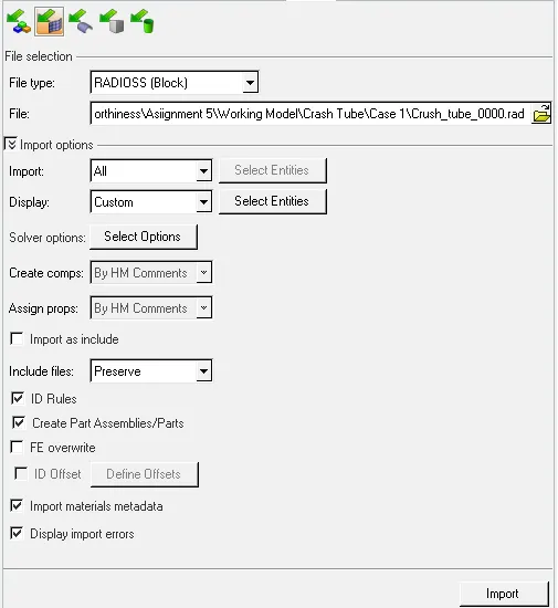
fig - Import the Files

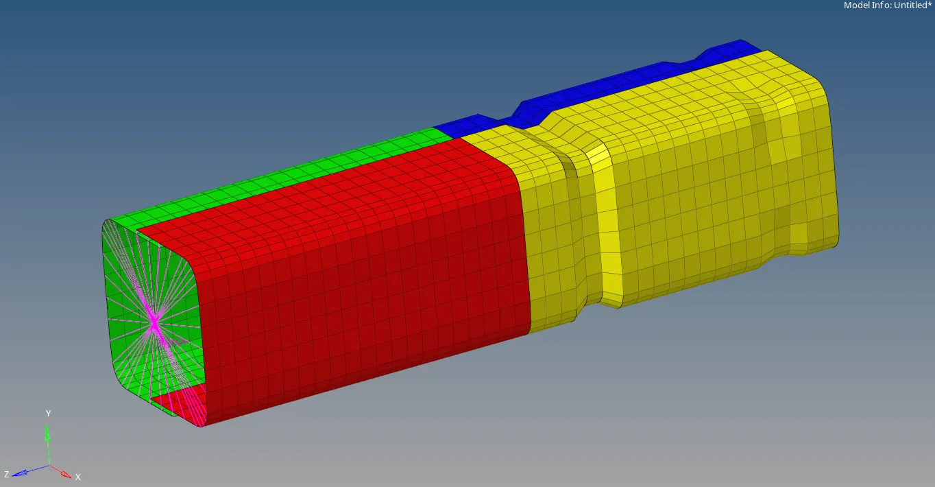
fig - Imported Model

Next, we check for component properties,

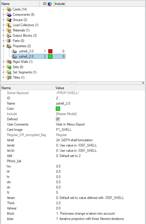
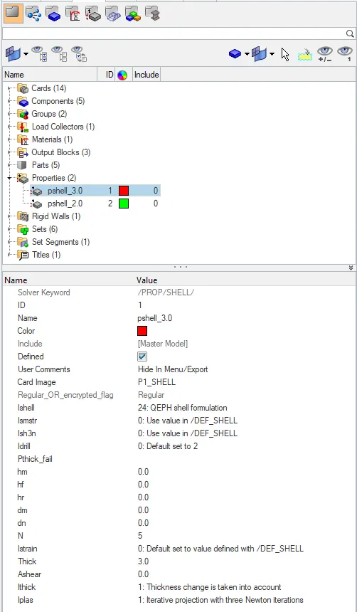
We also check the type of contact available in the model and its properties,

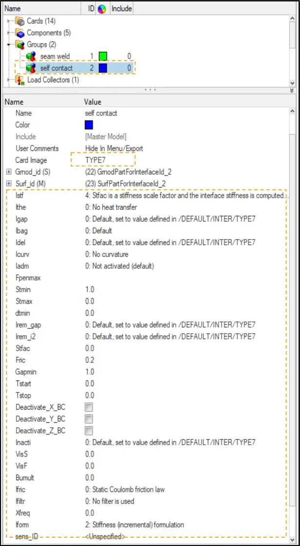
Here we can see that the type of contact used is Type 7 and its properties are kept to default.

After checking the model properties next step is to run the radios and check the radios out a file to see what is the energy error and hourglass energy and also the simulation time.

fig - Saving the model as

Radios Out-File Results:

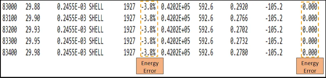
From the above image of radios out the file, we can say that energy error is within the acceptable range so we can go ahead with the result of energies and plot them. Energy Error is -3.8%.

Rigid Wall Force Plot:

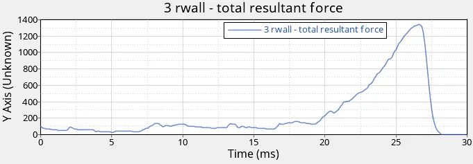
Here we can see that the rigid wall force is increasing suddenly after 20 sec this is because after 20 sec we can observe that the more elements coming into the contacts of each other due to compression of the crash tube leading to rising in the resultant force.

Rigid Wall Force is around 1400N.

Contact Force:

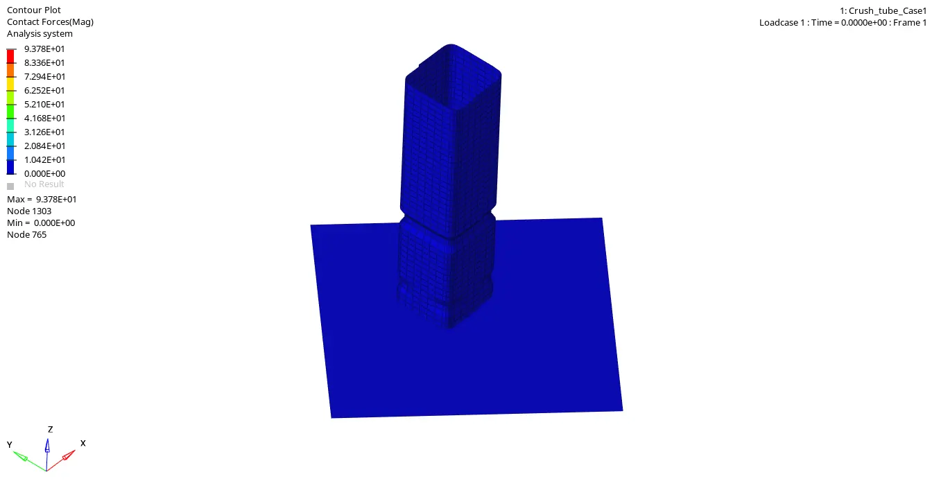
After 20 sec the contact between the slave elements and the master element is increasing leading to rising in the contact force and its interface.

Contact Force is around 93.7N.

Internal Energy Plot:

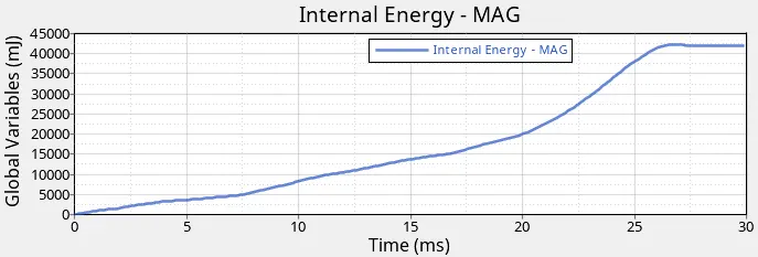
From the above image we can see that internal energy is rising to 26 sec around after that it becomes constant. Till this point, it was increasing because the element was in contact with each other and the tube was under the compression action. after 26 sec the element is no more able to hold more internal energy because the tube is already been compressed to its max level and hereafter it cannot be compressed anymore. The animation can be seen above in the contact force.

Internal Energy is around 43000mJ.

TH/Part:

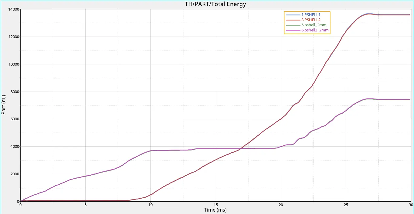
Here we have 4 curves representing 2 curves for 2mm thin tube and another one with 3 mm thin of the tube. When the tube impacts the bottom region there is a rise in the total energy of the bottom portion of the tube and stress concentration is also found to be more near the bottom area. As soon as the bottom portion reaches its max. compression limit then the upper portion of the tube starts getting compress and simultaneously there is a rise in the total energy of the tube. After this is seen to some more compression in the tube and due to this both the curves are found to be increasing simultaneously and the difference is due to the capacity of holding the energy.

All Energy:

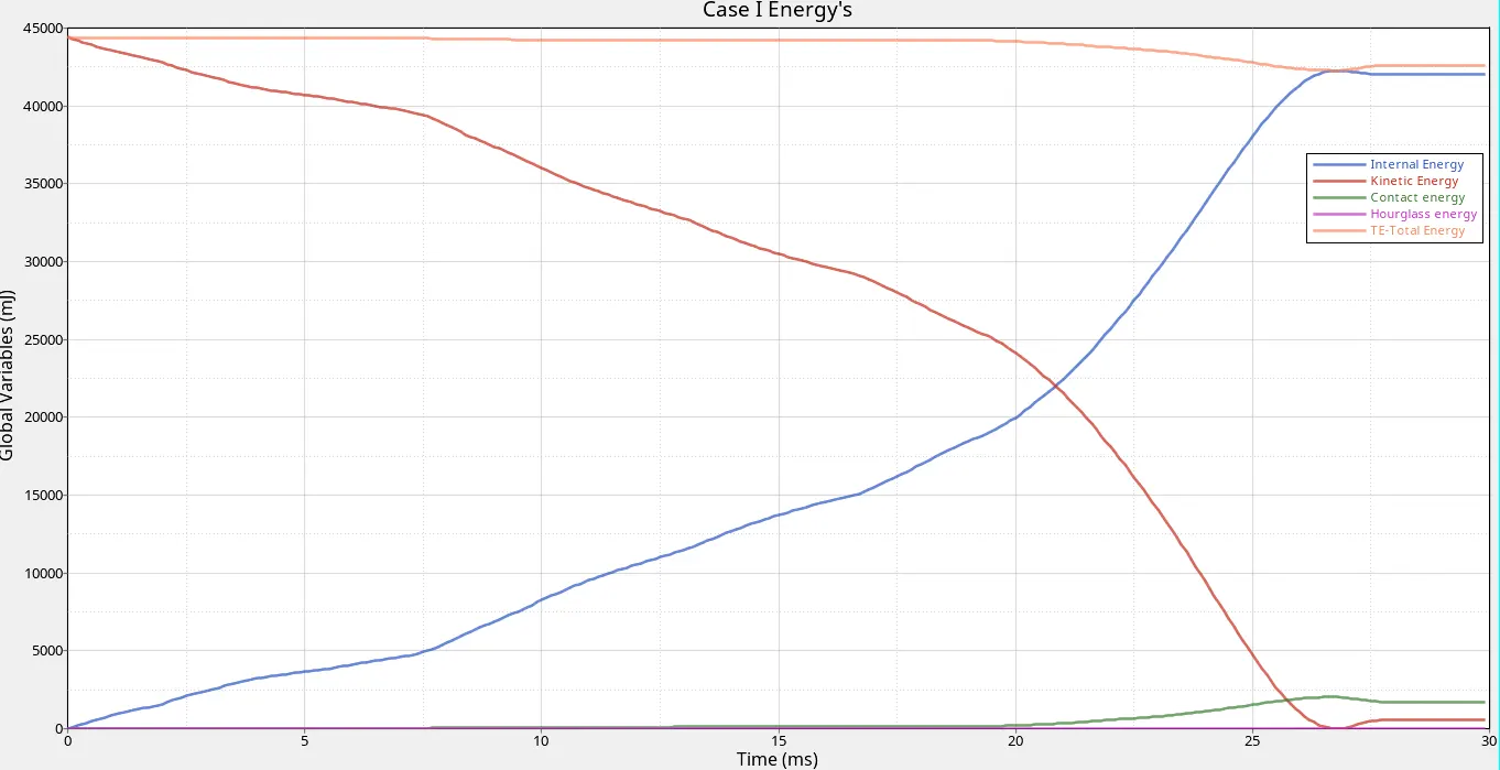
Here we can see that the kinetic and internal energy showing the opposite curve. This is because when there is impact or contact there is a reduction in the kinetic energy and simultaneously an increase in the internal energy. After the 20s we can see that there is contact force developing in the components due to which there is a rise in the contact energy of the component and the sake instant there is a reduction in the total energy due to this loss of energy.

Case II - Change the Inacti=6 and run

In this case, we import the same model as that of 1st case but this time we have to change the value of Inacti. So the question is what is this Inacti? So again to revise this is,

Inacti - Action to take if initial penetrations exist. Mean that if there is any initial penetration present in the model between the slave node and master node then this term will help to remove these initial penetration. As per the theory the recommended value for Inacti = 6 so that it helps in the removal of initial penetration in a better way than others.

So now we will apply the value in the model as shown below,

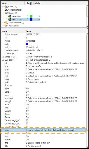
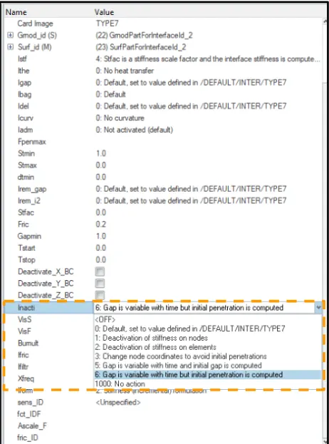
Above you can see that under the interface (Group) there is self contact interface available under which there is term inacti available. There is numerous option available to choose the value but we have set it to inacti = 6 because in this case the gap will vary with time but the initial penetration will be computed.

The next step is to run the radios and check the radios out a file to see what is the energy error and hourglass energy and also the simulation time.

fig - Saving the model as

Radios Out-File Results:

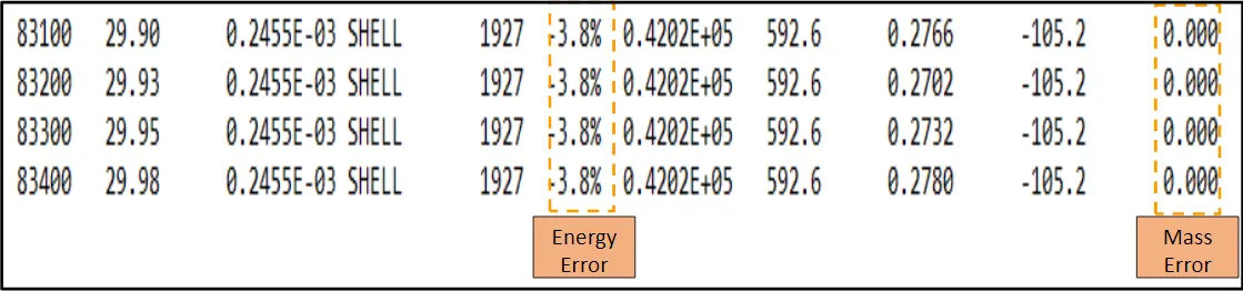
From the above image of radios out the file, we can say that energy error is within the acceptable range so we can go ahead with the result of energies and plot them. Energy Error is -3.8%.

Rigid Wall Force Plot:

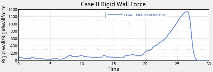
Here we can see that the rigid wall force is increasing suddenly after 20 sec this is because after 20 sec we can observe that the more elements coming into the contacts of each other due to compression of the crash tube leading to rising in the resultant force.

Rigid Wall Force is around 1380N

Contact Force:

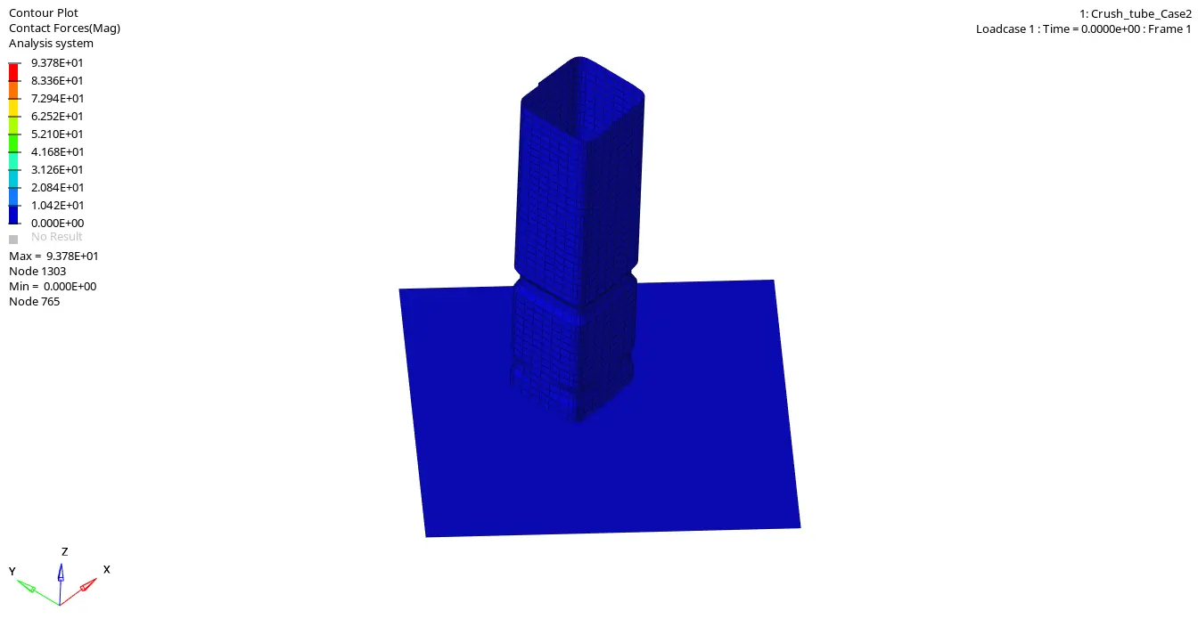
After 20 sec the contact between the slave elements and the master element is increasing leading to rising in the contact force and its interface.

Contact Force is around 93.7N.

Internal Energy Plot:

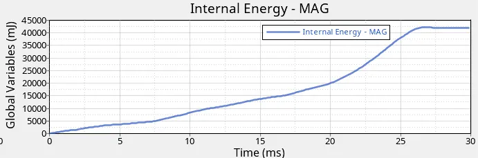
From the above image we can see that internal energy is rising to 26 sec around after that it becomes constant. Till this point, it was increasing because the element was in contact with each other and the tube was under the compression action. after 26 sec the element is no more able to hold more internal energy because the tube is already been compressed to its max level and hereafter it cannot be compressed anymore. The animation can be seen above in the contact force.

Internal Energy is around 43000mJ.

TH/Part:

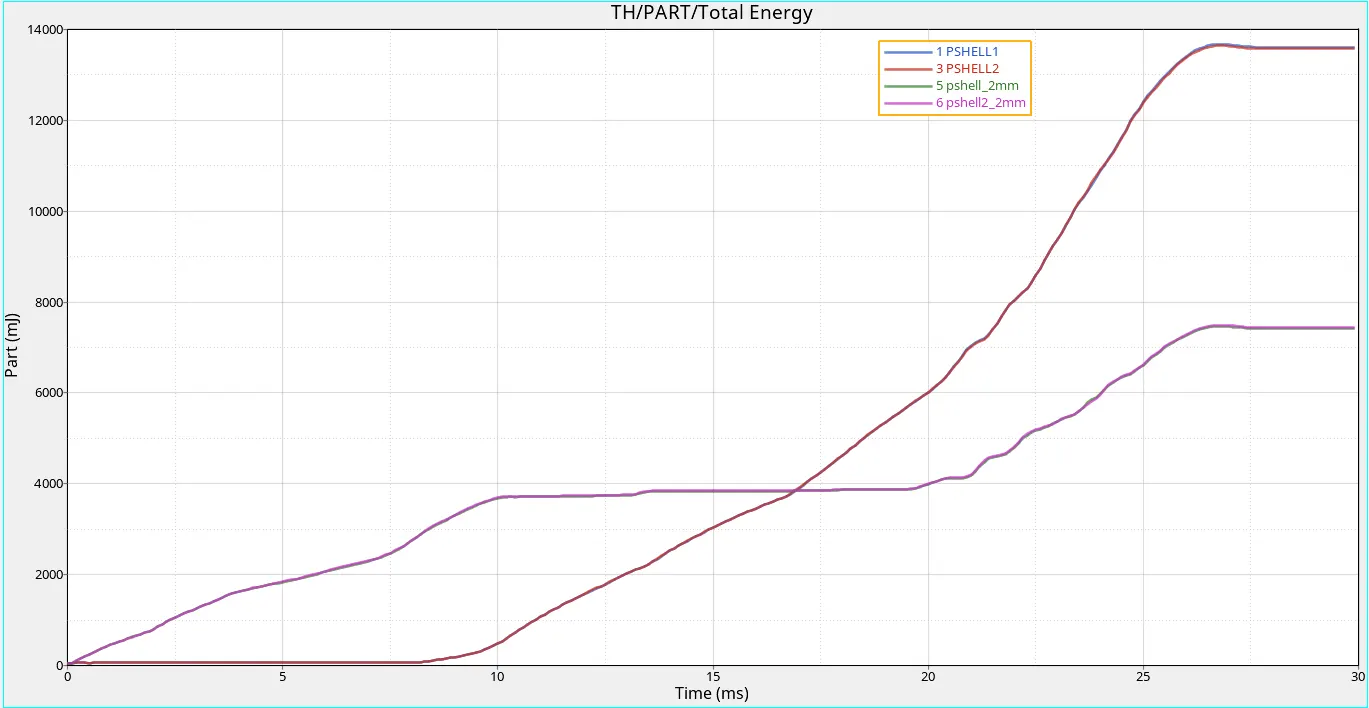
Here we have 4 curves representing 2 curves for 2mm thin tube and another one with 3 mm thin of the tube. When the tube impacts the bottom region there is a rise in the total energy of the bottom portion of the tube and stress concentration is also found to be more near the bottom area. As soon as the bottom portion reaches its max. compression limit then the upper portion of the tube starts getting compress and simultaneously there is a rise in the total energy of the tube. After this is seen to some more compression in the tube and due to this both the curves are found to be increasing simultaneously and the difference is due to the capacity of holding the energy.

All Energy:

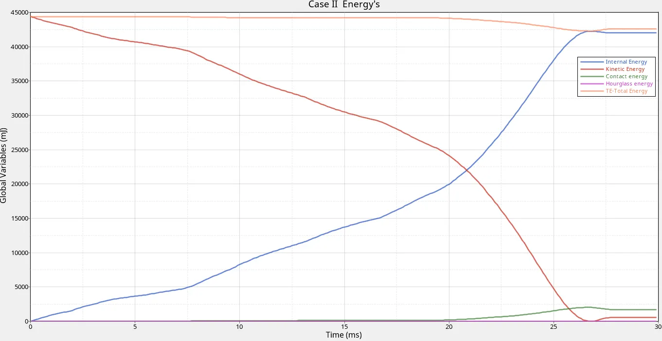
Here we can see that the kinetic and internal energy showing the opposite curve. This is because when there is impact or contact there is a reduction in the kinetic energy and simultaneously an increase in the internal energy. After the 20s we can see that there is contact force developing in the components due to which there is a rise in the contact energy of the component and the sake instant there is a reduction in the total energy due to this loss of energy.

Case III - Create the type 11 contact and run

In this case, we import the same model as that of 1st case but this time we have to add the type 11 interface that is it will be the combined case of Type 7 and Type 11 also can be said as Type 19. As discussed above Type 11 is used to define the edge to edge contact and is almost the same as type 7. So will see the type 11 card here,

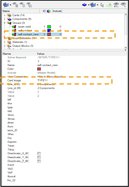
Under the group, we created oneself contact and change the card image to type 11. The value is kept as it is the simulation that is run to observe the result.

After adding the self-contact card next step is to run the radios and check the radios out a file to see what is the energy error and hourglass energy and also the simulation time.

fig - Saving the model as

Radios Out-File Results:

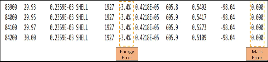
From the above image of radios out the file, we can say that energy error is within the acceptable range so we can go ahead with the result of energies and plot them. Energy Error is -3.4%.

Rigid Wall Force Plot:

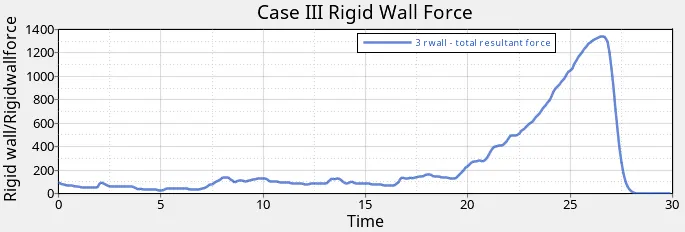
Here we can see that the rigid wall force is increasing suddenly after 20 sec this is because after 20 sec we can observe that the more elements coming into the contacts of each other due to compression of the crash tube leading to rising in the resultant force.

Rigid Wall Force is around 1380N

Contact Force:

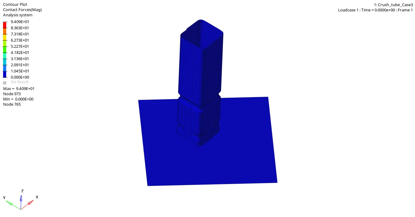
After 20 sec the contact between the slave elements and the master element is increasing leading to rising in the contact force and its interface.

Contact Force is around 94N.

Internal Energy Plot:

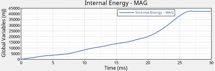
From the above image we can see that internal energy is rising to 26 sec around after that it becomes constant. Till this point, it was increasing because the element was in contact with each other and the tube was under the compression action. after 26 sec the element is no more able to hold more internal energy because the tube is already been compressed to its max level and hereafter it cannot be compressed anymore. The animation can be seen above in the contact force.

Internal Energy is around 43000mJ.

TH/Part:

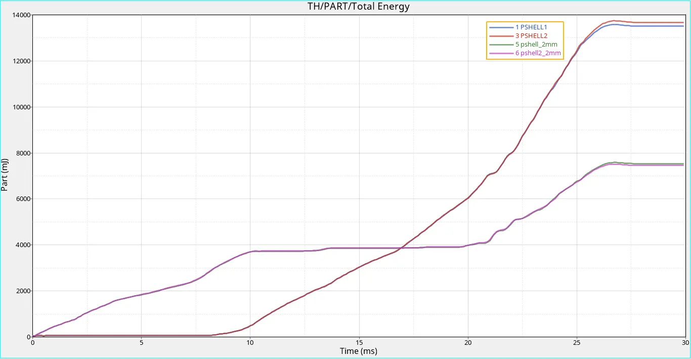
Here we have 4 curves representing 2 curves for 2mm thin tube and another one with 3 mm thin of the tube. When the tube impacts the bottom region there is a rise in the total energy of the bottom portion of the tube and stress concentration is also found to be more near the bottom area. As soon as the bottom portion reaches its max. compression limit then the upper portion of the tube starts getting compress and simultaneously there is a rise in the total energy of the tube. After this is seen to some more compression in the tube and due to this both the curves are found to be increasing simultaneously and the difference is due to the capacity of holding the energy.

All Energy:

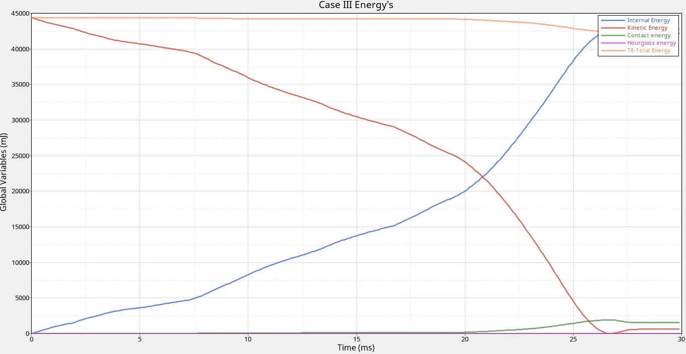
Here we can see that the kinetic and internal energy showing the opposite curve. This is because when there is impact or contact there is a reduction in the kinetic energy and simultaneously an increase in the internal energy. After the 20s we can see that there is contact force developing in the components due to which there is a rise in the contact energy of the component and the sake instant there is a reduction in the total energy due to this loss of energy.

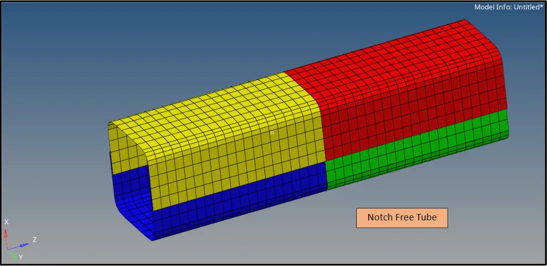
Case IV - Remove both notches and remove boundary conditions on a rigid body node then run

In this case, we import the same model as that of the 1st case and remove the notches present in the model to observe the effect of removing the notches from the model.

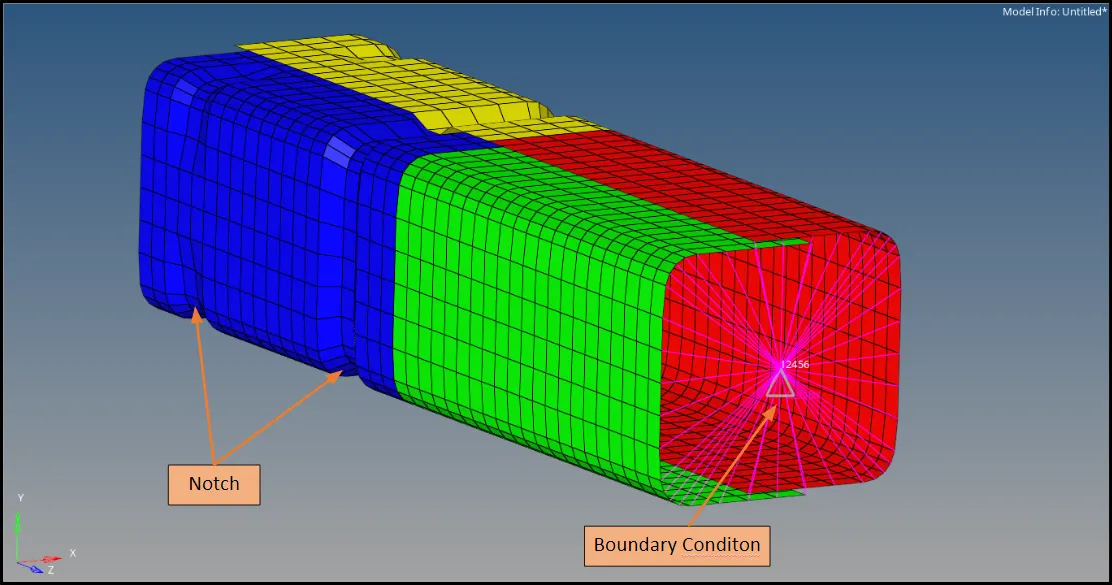
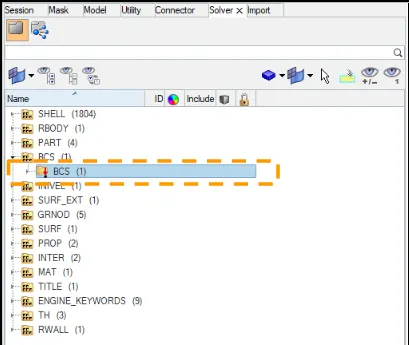
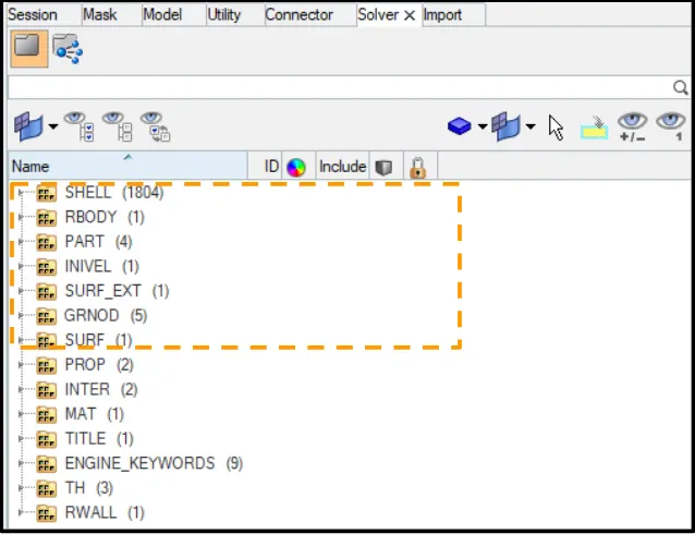
With BCS Without BCS

For removing the boundary condition we can go to solver - BCS (Boundary Condition) - Free all DOF from the constraint as shown above

After removing both the notch and boundary condition from the rigid wall from the tube next step is to run the radios and check the radios out a file to see what is its effect?

fig - Saving the model as

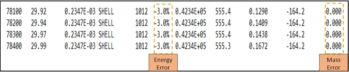
From the above image of radios out the file, we can say that energy error is within the acceptable range so we can go ahead with the result of energies and plot them. Energy Error is -3.0%.

Rigid Wall Force Plot:

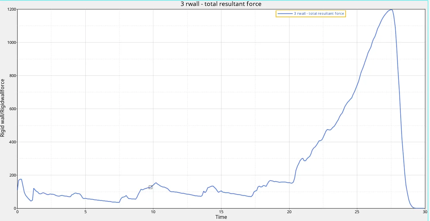
Here we can see that the rigid wall force is increasing suddenly after 20 sec this is because after 20 sec we can observe that the more elements coming into the contacts of each other due to compression of the crash tube leading to rising in the resultant force.

Rigid Wall Force is around 1200N

Contact Force:

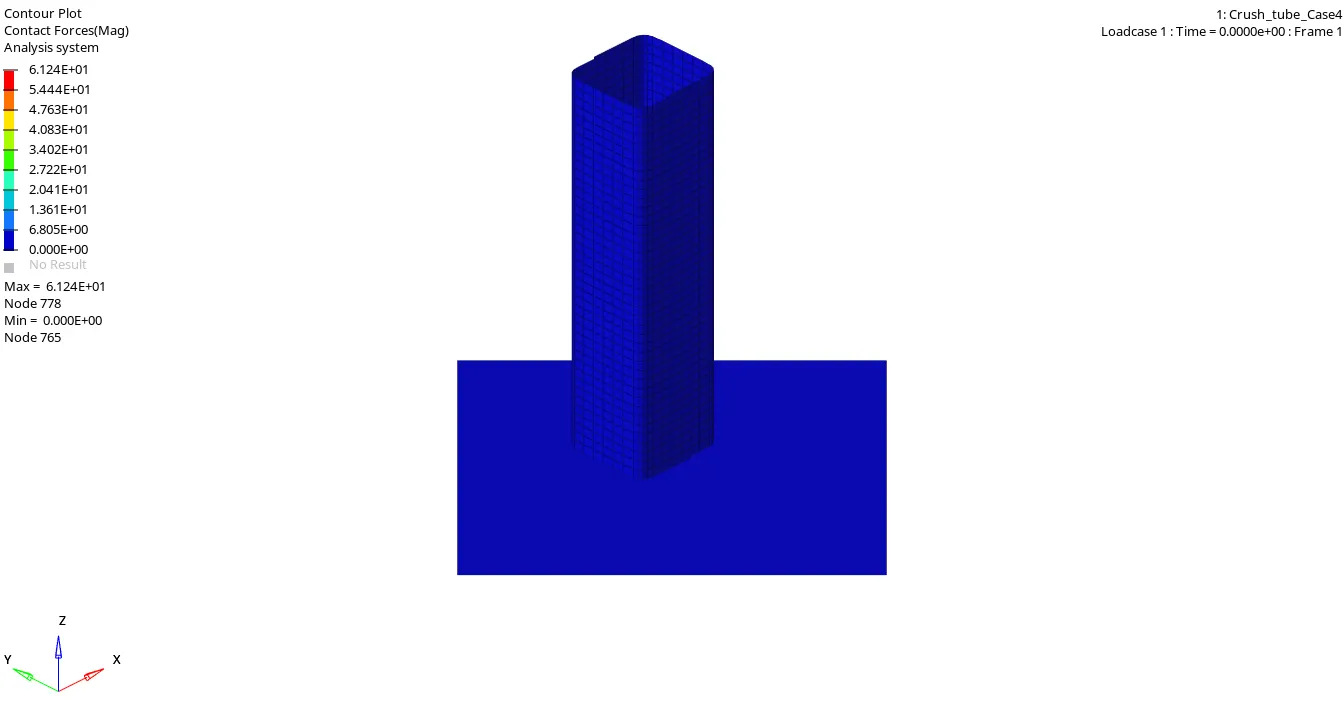
After 20 sec the contact between the slave elements and the master element is increasing leading to rising in the contact force and its interface. Here the contact force generated is less compared to all the other cases because there is no constraint to the tube in any of the directions as the rigid wall boundary condition is removed from the rigid wall and the tube is free to move or deform in all the directions.

Contact Force is around 61N.

Internal Energy Plot:

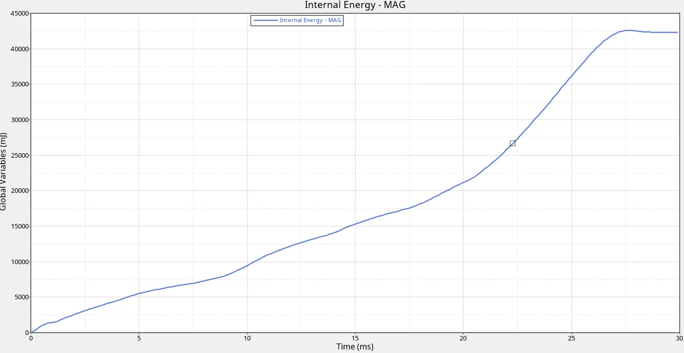
From the above image we can see that internal energy is rising to 26 sec around after that it becomes constant. Till this point, it was increasing because the element was in contact with each other and the tube was under the compression action. after 26 sec the element is no more able to hold more internal energy because the tube is already been compressed to its max level and hereafter it cannot be compressed anymore. The animation can be seen above in the contact force.

Internal Energy is around 43000mJ.

TH/Part:

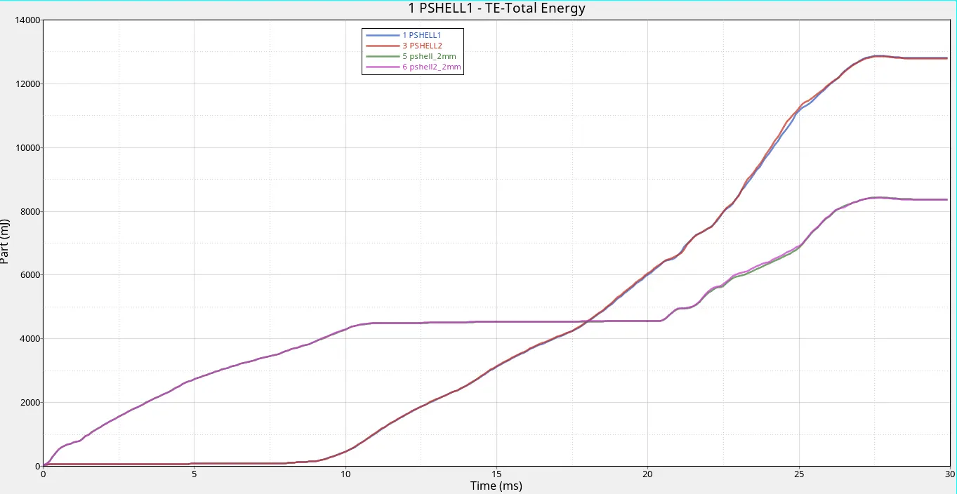
Here we have 4 curves representing 2 curves for 2mm thin tube and another one with 3 mm thin of the tube. When the tube impacts the bottom region there is a rise in the total energy of the bottom portion of the tube and stress concentration is also found to be more near the bottom area. As soon as the bottom portion reaches its max. compression limit then the upper portion of the tube starts getting compress and simultaneously there is a rise in the total energy of the tube. After this is seen to some more compression in the tube and due to this both the curves are found to be increasing simultaneously and the difference is due to the capacity of holding the energy.

All Energy:

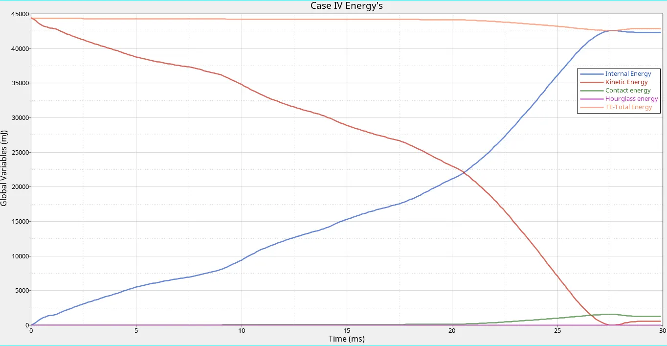
Here we can see that the kinetic and internal energy showing the opposite curve. This is because when there is impact or contact there is a reduction in the kinetic energy and simultaneously an increase in the internal energy. After the 20s we can see that there is contact force developing in the components due to which there is a rise in the contact energy of the component and the sake instant there is a reduction in the total energy due to this loss of energy.

Case V - Create a new notch in the middle, select the whole section, and run

In this case, we import the same model as that of the 1st case and create a notch in the middle of the model.

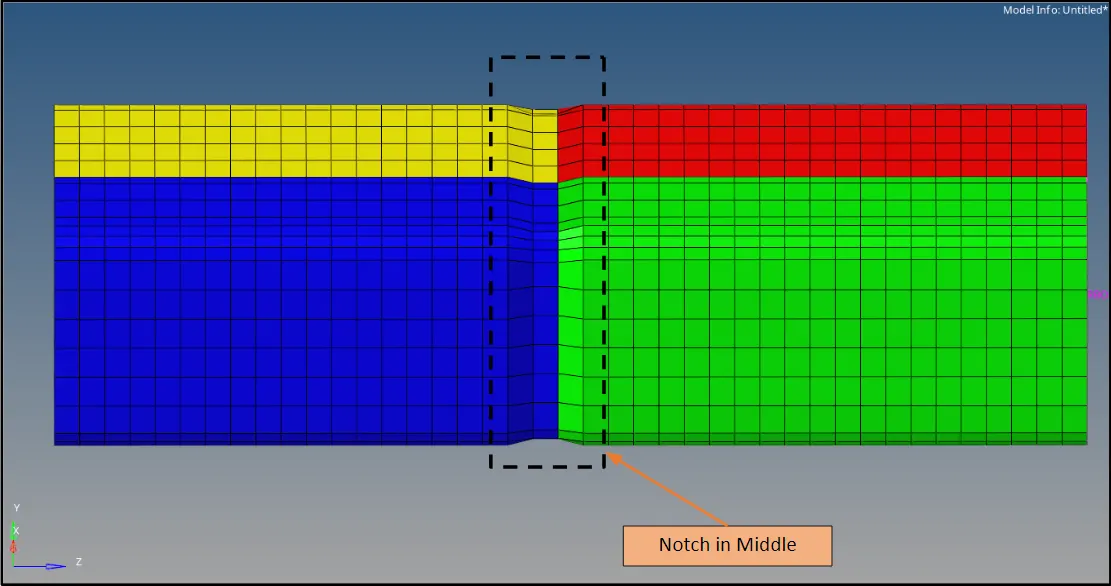
After creating the notch in the middle of the tube next step is to run the radios and check the radios out a file to see what is its effect creating the notch in the middle of the tube.

fig - Saving the model as

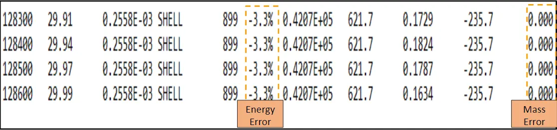
From the above image of radios out the file, we can say that energy error is within the acceptable range so we can go ahead with the result of energies and plot them. Energy Error is -3.3%.

Rigid Wall Force Plot:

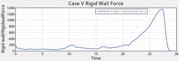
Here we can see that the rigid wall force is increasing suddenly after 20 sec this is because after 20 sec we can observe that the more elements coming into the contacts of each other due to compression of the crash tube leading to rising in the resultant force.

Rigid Wall Force is around 1300N

Contact Force:

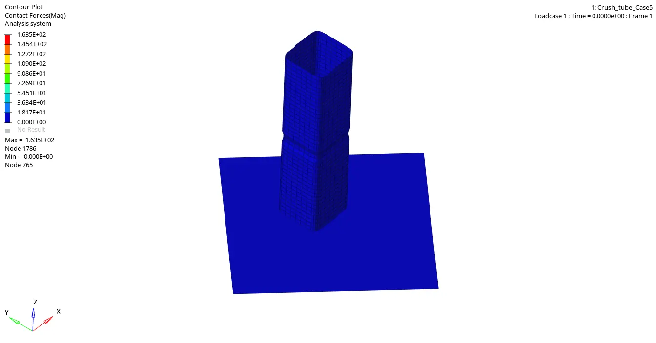
After 20 sec the contact between the slave elements and the master element is increasing leading to rising in the contact force and its interface. In this case, as the notch is in the middle of the tube the stress concentration can be seen along the middle of the tube near the notch. More number of elements are coming into contact that is why there is a slight increase in the contact force and energy.

Contact Force is around 163 N.

Internal Energy Plot:

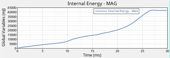
From the above image we can see that internal energy is rising to 26 sec around after that it becomes constant. Till this point, it was increasing because the element was in contact with each other and the tube was under the compression action. after 26 sec the element is no more able to hold more internal energy because the tube is already been compressed to its max level and hereafter it cannot be compressed anymore. The animation can be seen above in the contact force.

Internal Energy is around 43000mJ.

TH/Part:

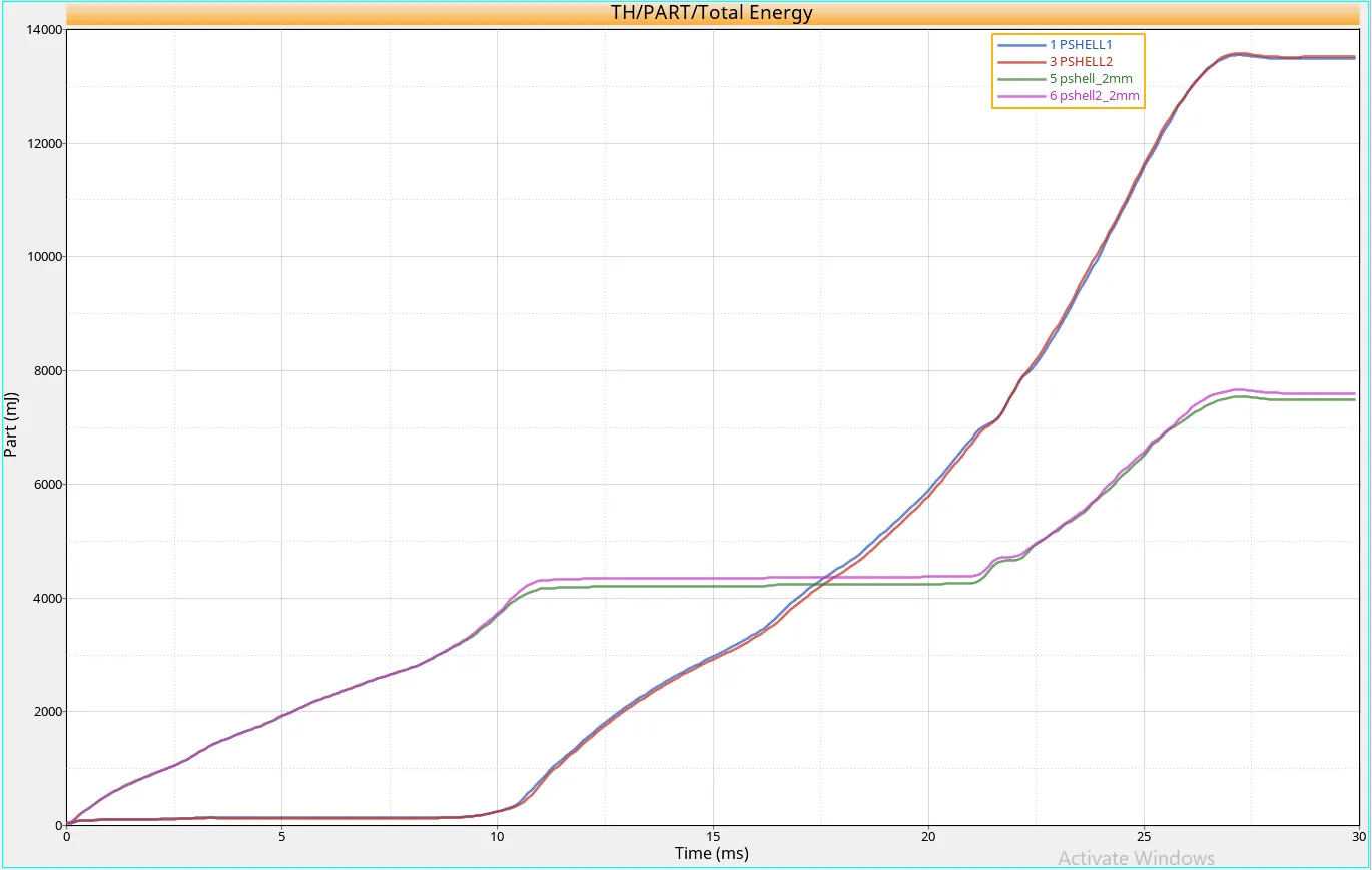
Here we have 4 curves representing 2 curves for 2mm thin tube and another one with 3 mm thin of the tube. When the tube impacts the bottom region there is a rise in the total energy of the bottom portion of the tube and stress concentration is also found to be more near the bottom area. As soon as the bottom portion reaches its max. compression limit then the upper portion of the tube starts getting compress and simultaneously there is a rise in the total energy of the tube. After this is seen to some more compression in the tube and due to this both the curves are found to be increasing simultaneously and the difference is due to the capacity of holding the energy.

All Energy:

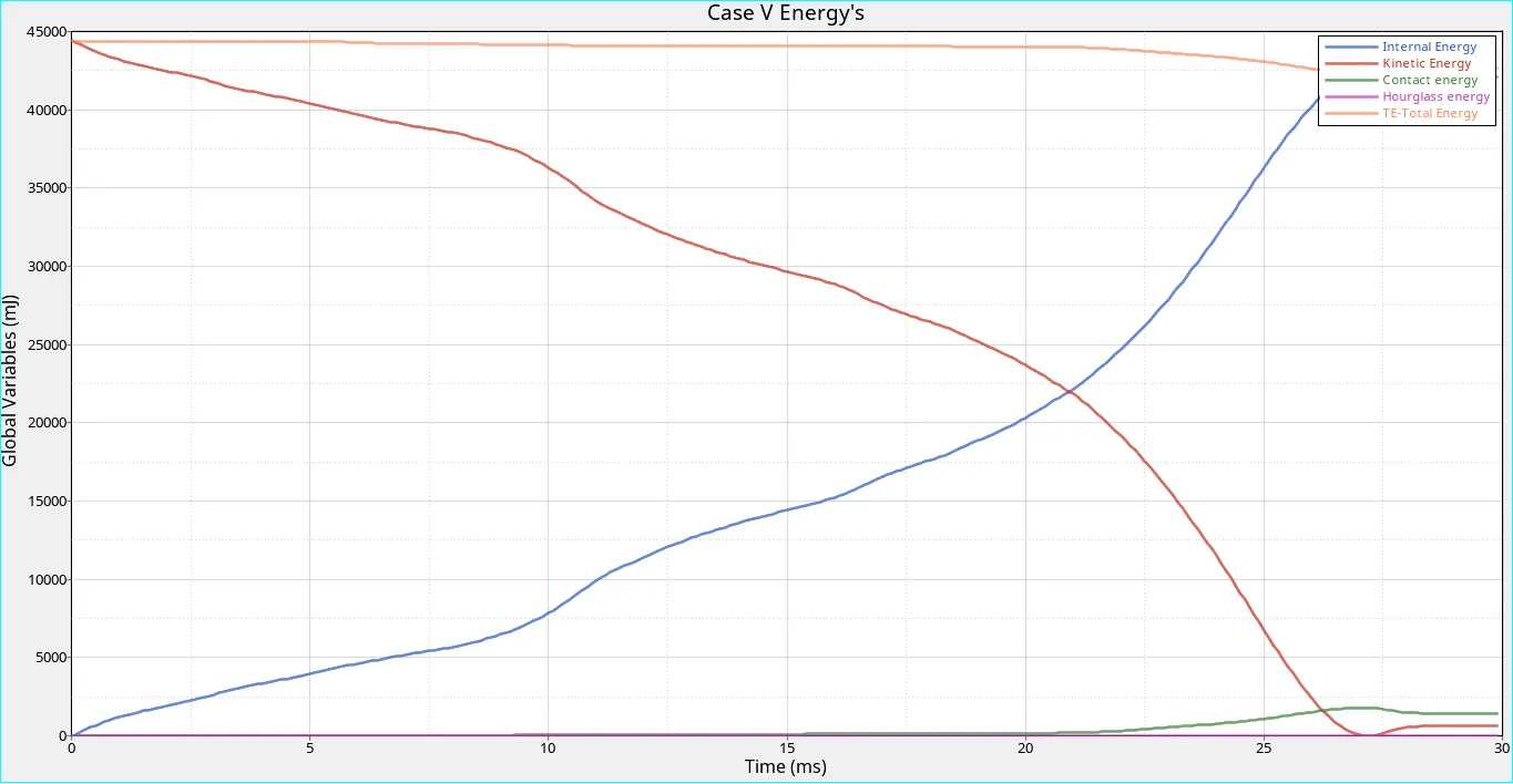
Here we can see that the kinetic and internal energy showing the opposite curve. This is because when there is impact or contact there is a reduction in the kinetic energy and simultaneously an increase in the internal energy. After the 20s we can see that there is contact force developing in the components due to which there is a rise in the contact energy of the component and the sake instant there is a reduction in the total energy due to this loss of energy.

Case VI - Create a new notch with nodes only from opposing 2 faces and run

In this case, we import the same model as that of the 1st case and create a notch on two opposite faces as shown below,

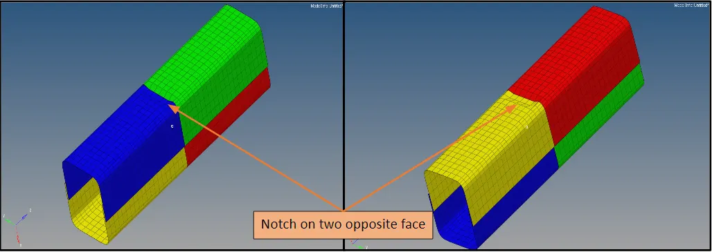
After creating the notch on two opposite faces of the tube next step is to run the radios and check the radios out a file to see what is its effect creating the notch in the middle of the tube.

fig - Saving the model as

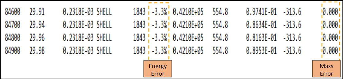
From the above image of radios out the file, we can say that energy error is within the acceptable range so we can go ahead with the result of energies and plot them. Energy Error is -3.3%.

Rigid Wall Force Plot:

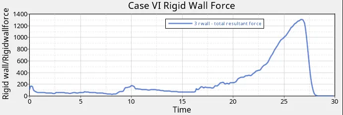
Here we can see that the rigid wall force is increasing suddenly after 20 sec this is because after 20 sec we can observe that the more elements coming into the contacts of each other due to compression of the crash tube leading to rising in the resultant force.

Rigid Wall Force is around 1300N

Contact Force:

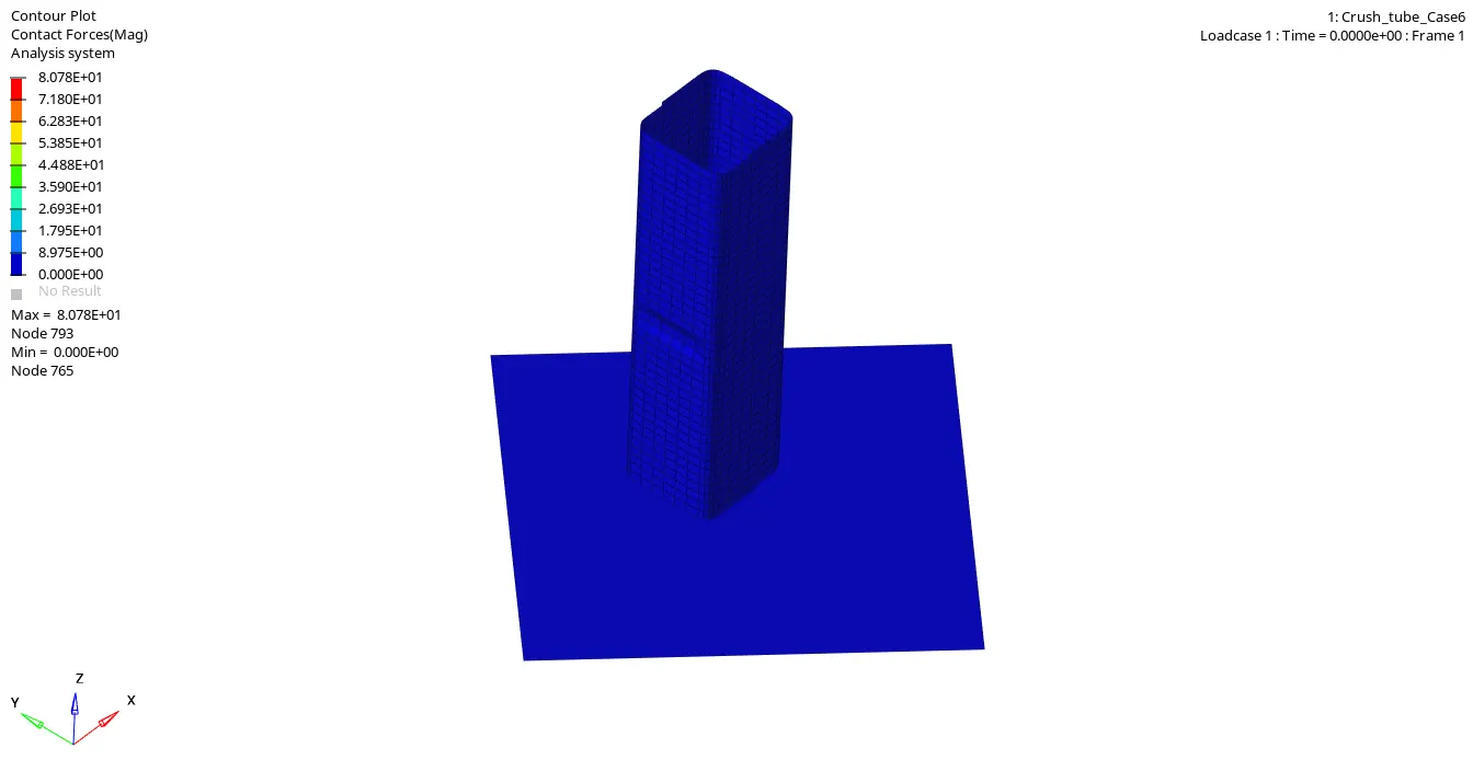
After 20 sec the contact between the slave elements and the master element is increasing leading to rising in the contact force and its interface. Here we can see that due to a decrease in the notch in on the opposite face there is a reduction in the contact force.

Contact Force is around 80.7N.

Internal Energy Plot:

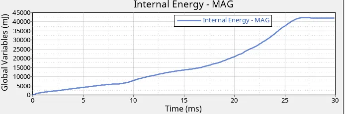
From the above image we can see that internal energy is rising to 26 sec around after that it becomes constant. Till this point, it was increasing because the element was in contact with each other and the tube was under the compression action. after 26 sec the element is no more able to hold more internal energy because the tube is already been compressed to its max level and hereafter it cannot be compressed anymore. The animation can be seen above in the contact force.

Internal Energy is around 43000mJ.

TH/Part:

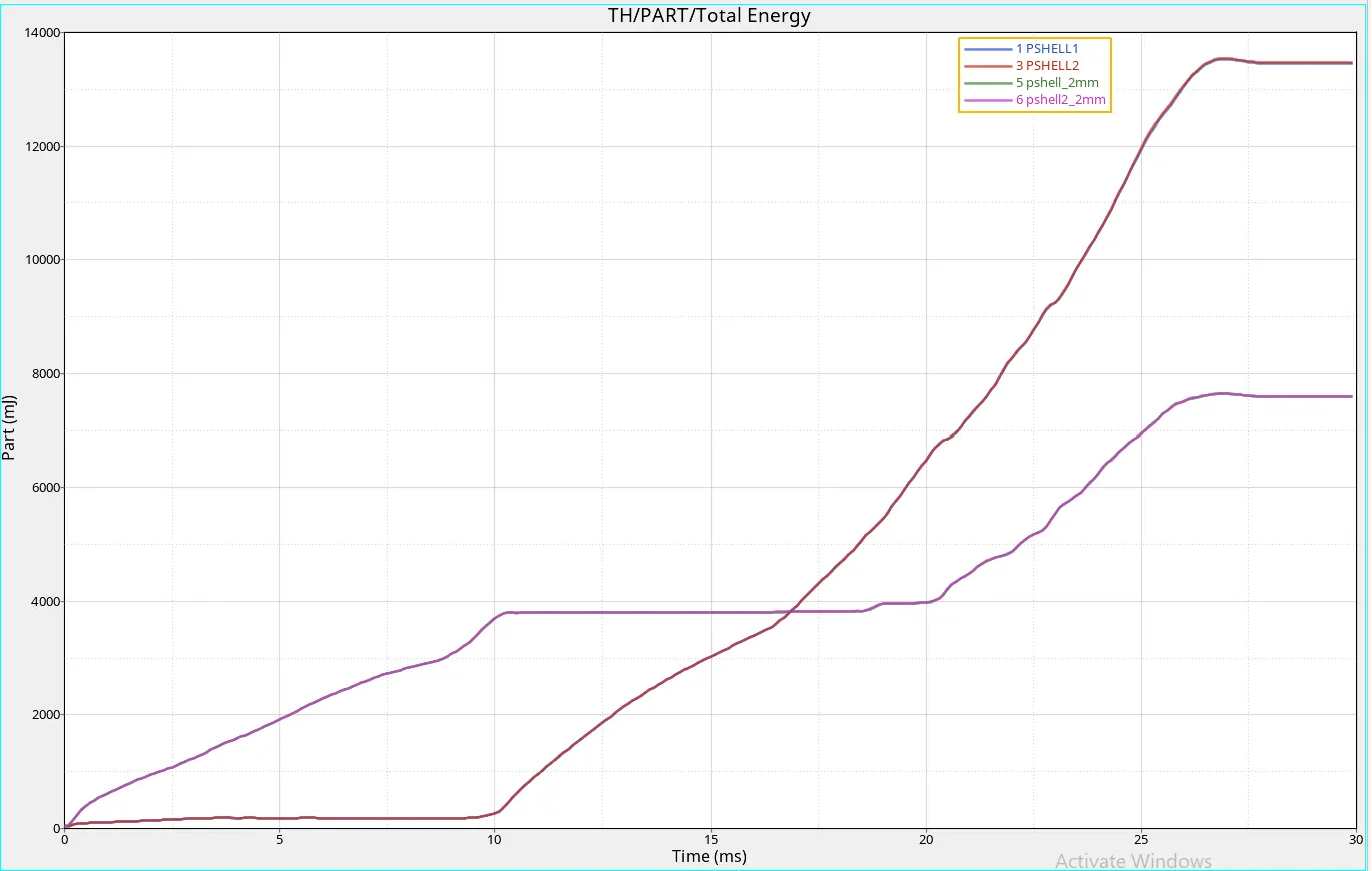
Here we have 4 curves representing 2 curves for 2mm thin tube and another one with 3 mm thin of the tube. When the tube impacts the bottom region there is a rise in the total energy of the bottom portion of the tube and stress concentration is also found to be more near the bottom area. As soon as the bottom portion reaches its max. compression limit then the upper portion of the tube starts getting compress and simultaneously there is a rise in the total energy of the tube. After this is seen to some more compression in the tube and due to this both the curves are found to be increasing simultaneously and the difference is due to the capacity of holding the energy.

All Energy:

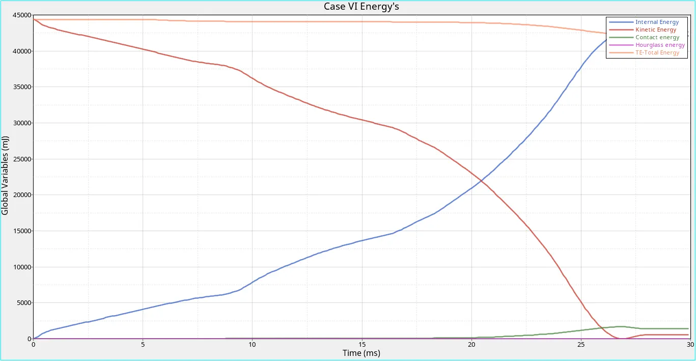
Here we can see that the kinetic and internal energy showing the opposite curve. This is because when there is impact or contact there is a reduction in the kinetic energy and simultaneously an increase in the internal energy. After the 20s we can see that there is contact force developing in the components due to which there is a rise in the contact energy of the component and the sake instant there is a reduction in the total energy due to this loss of energy.

Comparison between Internal Energy

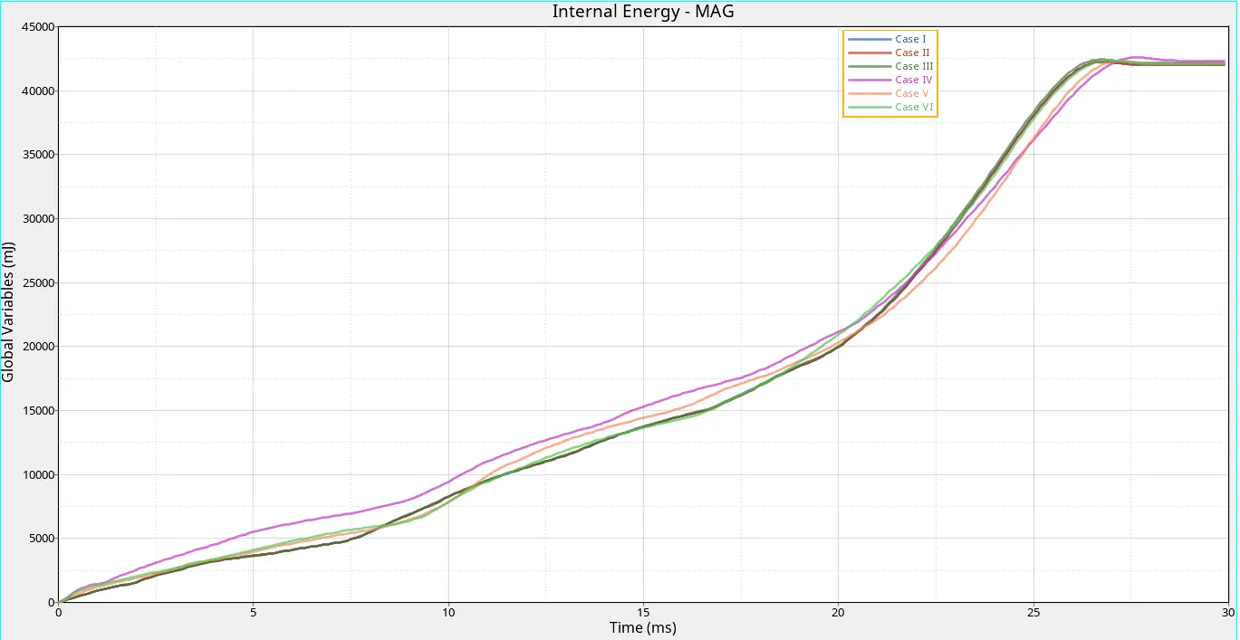
We split this plot into two sections to understand it well what is happening in this

Case I-III Comparison:

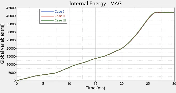
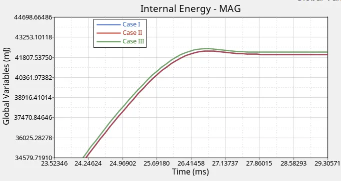
From the above plot, we can observe that case I and case II internal energy is coinciding with each other so there is no much difference between these two cases only due to a change in the inacti value. The difference in the internal energy is observed in case I, II, and case III as seen above in the 2nd plot after the zoom. As we know that in this case along with type 7 contact type 11 is also illustrated which uses complex algorithms in identifying the contact more appropriately between the edges and line. Due to this, there is slightly more internal energy observed in the tube.

Case IV-VI Comparison:

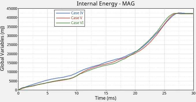
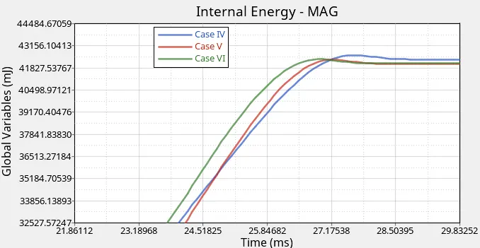
From the above plot, we can observe that at the end of the radios there is a difference in the internal energy of the tubes. This difference is studied in different ways after zooming the plot at the end of simulation to understand the difference well. There is a difference in the internal energy of Case IV and Case V, VI, this is because in case IV there tube is free to move along any direction as the rigid body boundary condition is removed. To make it sense more we have analyzed the case IV again by keeping the constraint on for tube and observed the below result.

Case VI Comparison with & without BCS:

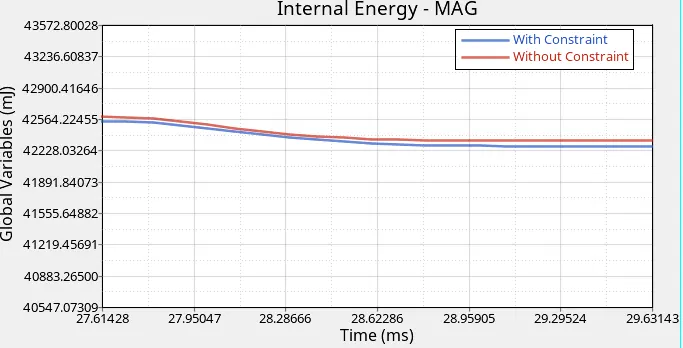
Here we can see the difference in the internal energy with and without constraint case. When there is no constraint present in the tube there is little more absorption of internal energy than compared to the constraint case. This difference is either due to deformation or buckling of the tube where the constraint is applied.

Comparison between Contact Energy

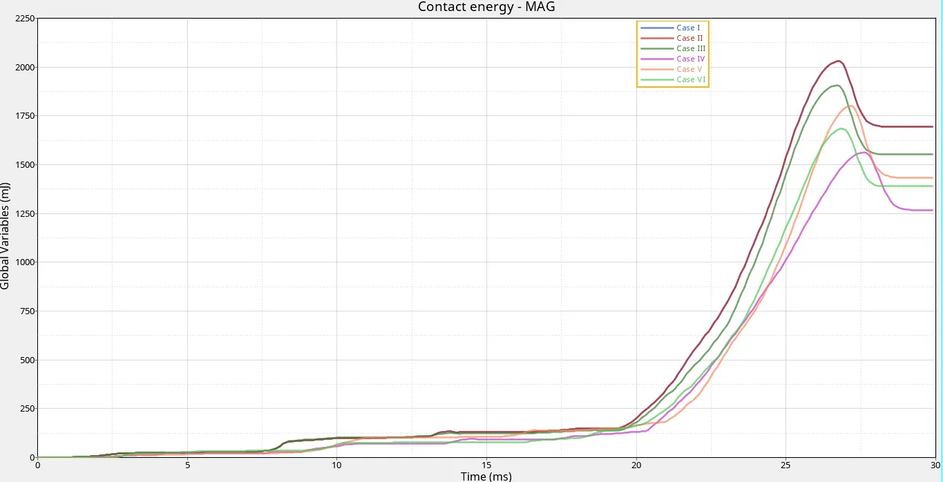
We split this plot into two sections to understand it well what is happening in this

Case I-III Comparison:

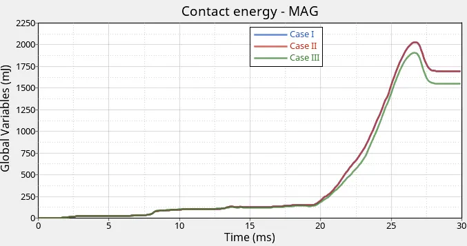
From the above plot, we can observe that case I and case II contact energy is coinciding with each other so there is no much difference between these two cases only due to a change in the inacti value. The difference in the contact energy is observed in case I, II, and case III as seen above in the plot. As we know that in this case along with type 7 contact type 11 is also illustrated which uses complex algorithms in identifying the contact more appropriately between the edges and line. Due to this, there is slightly more contact energy observed in the tube.

Case IV-VI Comparison:

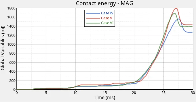
From the above plot, we can observe that at the end of the radios there is a difference in the contact energy of the tubes. There is a difference in the contact energy of Case IV and Case V, VI, this is because in case IV there tube is free to move along any direction as the rigid body boundary condition is removed. In case V the contact energy is more as there is a notch in the middle of the tube and due to t this the whole stress concentration was seen in the center of the tube. In case VI the contact energy is a little less than the case V as the notch is present on only two opposite faces of the tube where the less area will be in contact.

How does the notch affect the results?

• The notch effect stress concentration.
• The notch gives more deformation.
• The notch is affecting the overall internal energy and total energy.

Learning Outcomes:

• Study of different interfaces in HYPER-MESH & RADIOS.
• Creating the interface card in HYPERMESH.
• Effects of Penetration and Intersection.

Conclusion:

Here we can say that we can conclude the contact interface part of the component. Its effects and results with various types of contact. The results are compared and a brief explanation about each case is explained above in the report.