Crash Tube Analysis using Different types of Interfaces available in Radioss and Hypermesh workbench. 2D -1D element mesh deployment over the Bumper Assembly using Hypermesh.
Aim:- Crash Tube Analysis using Different types of Interfaces available in Radioss and Hypermesh workbench. 2D -1D element deployment over the Bumper Assembly using Hypermesh.
Objectives:
1) Deploy proper 2D mesh and 1D connection on Bumper Assembly.
2) set different types of Interface connection and RUN the simulation. Study the Graphs and output files generated from the simulation run.
3) Run the given crash tube model as it is with type 2 and type 7 Interface setup.
4) Run the same Crash tube model using Type 7 interface parameters as recommended one along with Inacti=6 and run.
5) Create the type 11 contact and Run it along with Type2 and Type 7 interfaces.
6) Create different sort Notches over the model body and study the impact of the notch and No-notch over the model.
-The first objective is to mesh the given Bumper assembly with a Target Length of 6mm and deploying proper 1d element over the assembly.
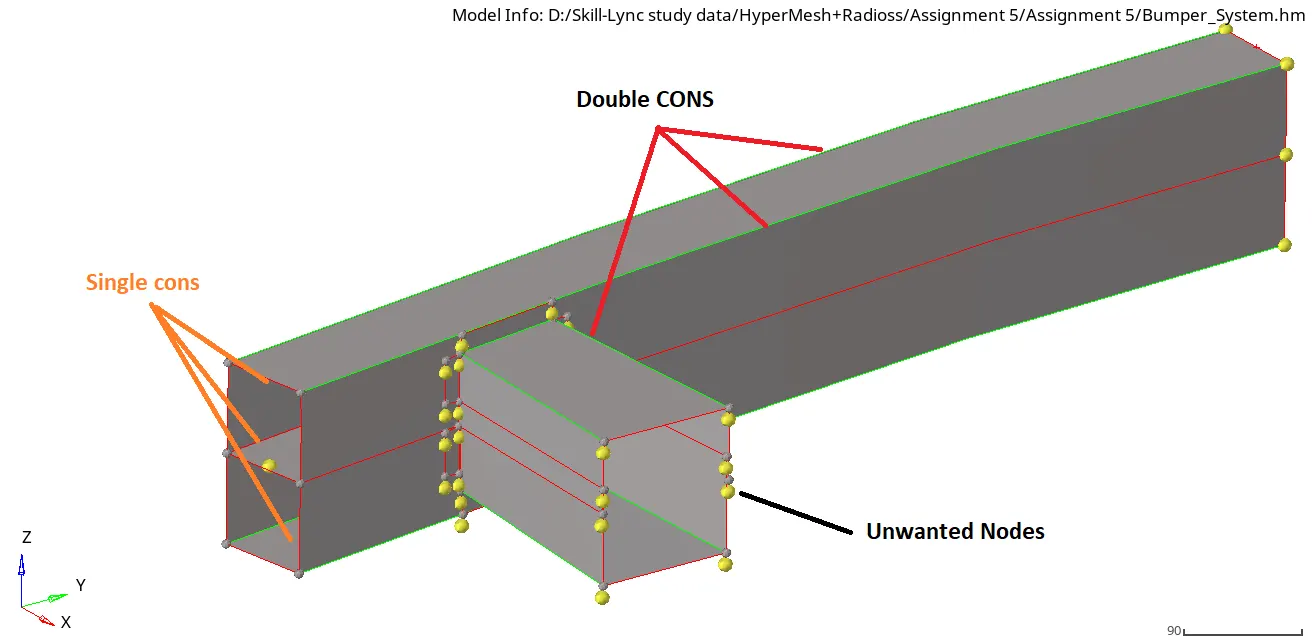
Fig 01
-The bumper assembly you can see in the above image has numbers of unwanted nodes and geometrical deformation. The Duble node at the edges indicates the connecting surfaces (Saved in different PIDs) and the Single CONs indicates the loose components or the free edges of the components.
-The first thing is to clear these errors in the model and do defeaturing where needed [NOTE: we don't have to extract mid surface as we get the model with Mid-surface extraction already done]
-Here are some screenshot showing geometrical cleanup
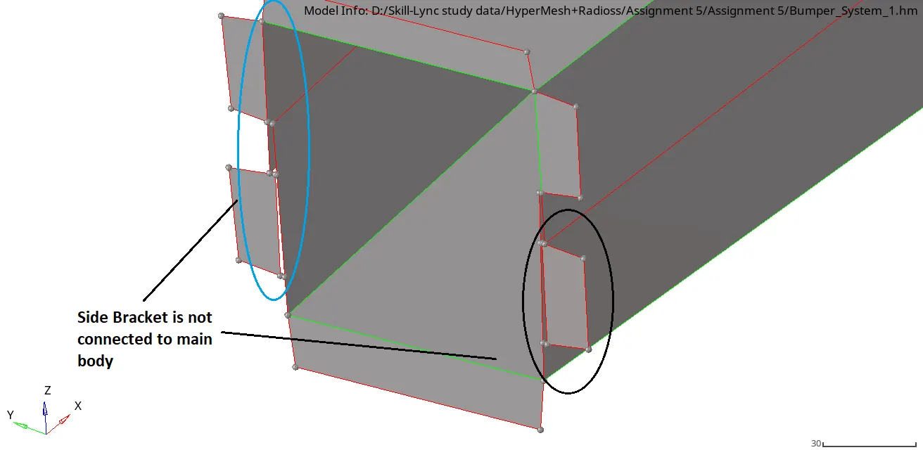
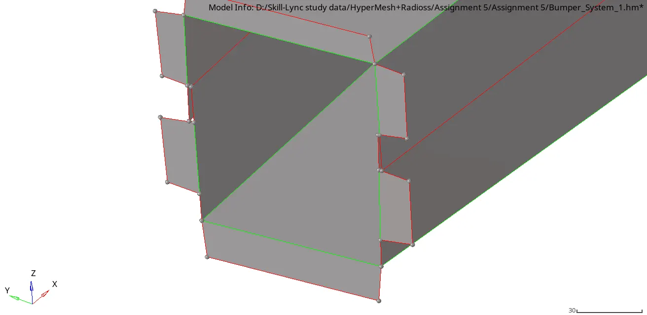
Before After
Fig 02
-As you can be observed in the above images that I had connected the braking surface to its actual geometry. I had used the "Surface Edit" option to perform this edge fixing. Other than that I had used the "quick edit" option from the "geom" Panel.
-After the Geometrical cleanup, I have moved forward with the meshing operation. Deployed the mesh of Target Length of 6mm over the parts using the "2D" mesh panel.
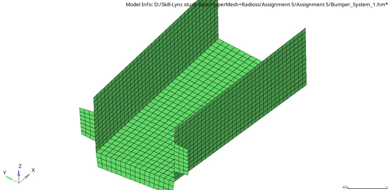
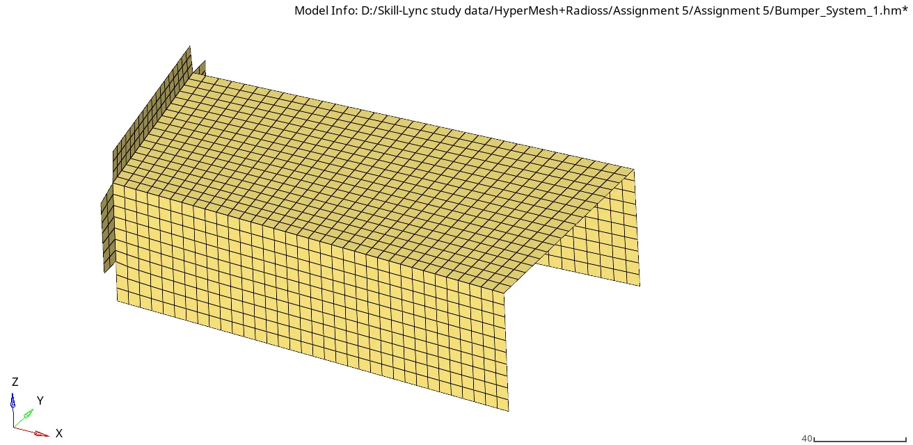
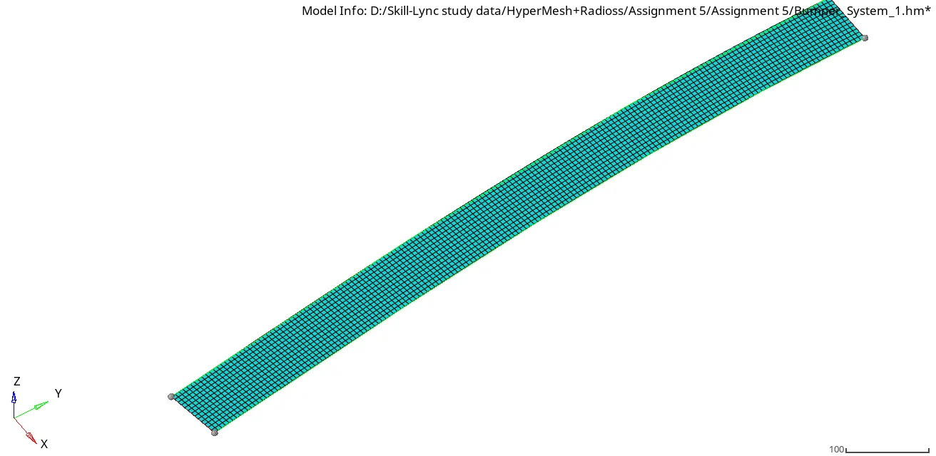
Fig 03
- After meshing check for the Quality criteria and move with the 1D element deployment. Here I had joint the surfaces using a "Seam" weld. The proper connection data is not provided so I asked my senior for the connection and from his suggestion I deployed seam weld connection over the meting parts.
- I had used the "1D" panel for this operation. The path is as " 1D --> connectors --> seam" and used seam panel for connection deployment.
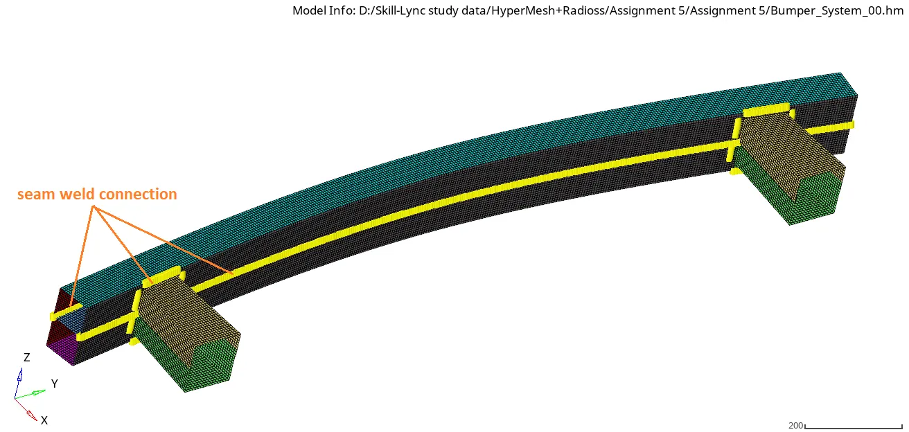
-The 1D connection only deployed where we see the free edge without any reference. For example, the middle plate has 4 free edges as you can see in Fig01 (Single cons), So it is necessary to restrict the motion of that plate otherwise it will create problems in further simulation. I had deployed the seam well with reference to upper and lower C-channel and make it as one structure. The color of the mesh is different because over each part because they are saved in different PIDs.
Interface Modeling
- Interfaces are defined to model how parts interact when they come into contact with each other.
- There are different methods that are available for Interface contact, but we are only going through some of the popular once that are widely used in the industries.
1) Penalty Method:-
-Treat the behavior between slave nodes and the Master segment as spring that generates resistive force as Penetration is happening. In this time step is inversely proportional to the stiffness.
Nodal time step
`Deltat <= sqrt((2M)/K)`
where M= mass of node
K= Stiffness (K interface + K element)
Kinematic Time Step
`Deltat <= 1/2 ((g-p)/((dp)/dt))`
where,
g = GAP value (imaginary boundary over the element wich having thickness same as the element)
p= Penetration value
dp/dt = Speed of sound in the material
-We should keep the thickness in check, if the Timestep decreases by a lot due to the increase in stiffness it will result in instability.
2)Type 7:- Node to surface contact.
-Its node to surface type contact with nonlinear stiffness. This stiffness non-linearity provides more stability during the simulation.
-A gap is defined around the master surface and slave nodes. Also, the cylindrical shape gap is formed near the edges to avoid irregular results near the edges. (Even though it's not suitable for edge to edge contact)
-The best thing about this contact it will able to simulate all types of impact in any direction.
-Auto impact simulation can possible with this contact.
-The main advantage of this contact is that the stiffness is not constant and increases with the penetration, preventing the nodes from going through the shell mid surface or penetrate the shell element.
Recommended [parameters under Type 7 contact
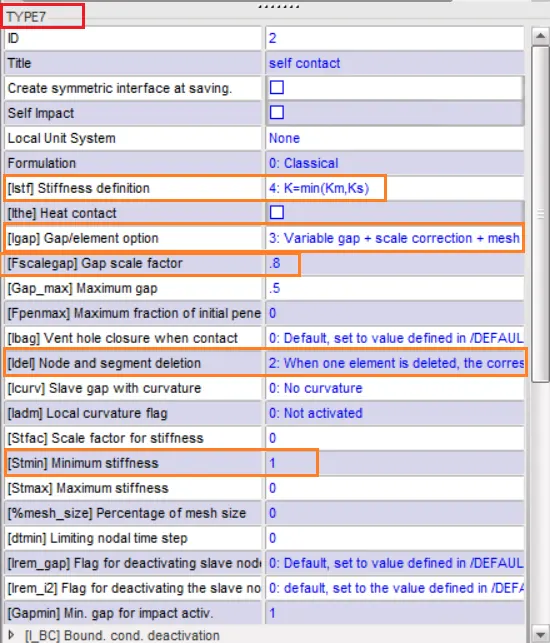
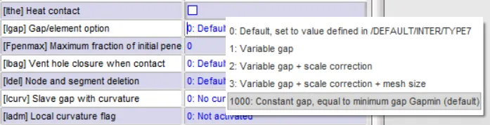
Igap :- Determine how the size of the gap is calculated, As you can see in the bottom image there are four options available under the Igap. Most probably using 2nd and 3rd options are considered as good practice. In most of the industrial cases, 3rd option is more preferable as it takes the gap, gap scale factor, and mesh size into consideration.
-0 only takes the Gapmin value into consideration which will lead to a false result in some cases. It's up the respective Engineer which type of Igap he should consider for a specific type of simulation
-3rd option is preferred because it will filter down the result as it takes three additional parameters into the considerations.
-Igap= 0, The gap is defined by Gapmin, and it's constant for all the contact.
-Igap=1, Gap varies and can be defined by the formula Igap= max[Gapmin,(gs+gm)], (where gs=ts/2 and gm=tm/2, ts largest thickness of shell connected slave and tm is the thickness of master shell)
-Igap=2, Variable calculated by Igap= max{Gapmin, min [Fscalegap * (gs +gm), % mesh size * (gs_l + gm_l), Gapmax]}
Gapmin:- It will define the Minimum gap for activation of the interface. Normally it will set up as 0.5.
-if we set Igap =0,1 or 2 and Gapmin also 0 (Default) it will take the min of the average thickness of the master shell element and half of the minimum element length. [Gapmin = min(tm, l/2)]
-Defining GAPmin is the best practice of all.
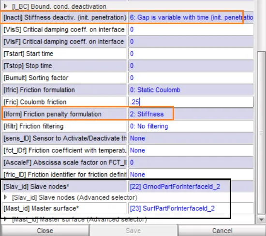
Inacti :- Determine the action to take if initial penetration exists. It dampened the initial penetration by allowing node some clearance over the GAP without activating the contact condition.
-There is a total of 0-6 flags available in the Iacti option but the 6th one is mostly used with Type 7 and Type 11 interface while 5th one is preferred best for Type 24.
Istf:- Initial Stiffness variable defined how the stiffness of the interface is calculated.
There are 0-5 flag available and 4th one [`K_0 = min (K_m, K_s)`] is considered best for the applications.
Km and Ks are the stiffness of the master surface and salve node and calculated in the backend.
Iform :- Determine the Friction formulation / sliding force calculation method.
There are two options that are available to calculate the sliding forces one is vicious and another is the Stiffness method.
the 2nd option preferred because as a result, it gives bigger time steps.
Stmin :- Min stiffness to used in the interface. It will set as 1000N.
Idel:- This option helps to stabilize the simulation by removing the contact condition from the element which will get fail and gets deleted from the model.
There are two options available,
1. When all elements associated with one segment are deleted, the segment is removed from the master side of the interface.
2. when one element is deleted all the corresponding segments get removed from the master aside of the interface.
2nd one is the best option because it will remove the master segment over the one deleted element which will stabilize the simulation to a great extend.
3) Type 11:- Edge to edge contact.
-All the parameters we learned inside the type 7 contact are the same here, the only difference is its represent edge to edge /Line to line contact.
-we can use this interface along with Type 7 for better results.
-Type 7 is good for surface and auto impact simulation but one drawback is it's not good with edge contact as its some time unable to recognize the contact itself.
4)Type 19:- Combination of Type 7 and Type 11 contact.
-All the parameters inside of type 7 and 11 can be easily available with this interface.
5) Type 24:- Node to surface and Surface to surface contact.
- This interface deploys the Single surface. surface to surface or node to surface contact interface using the penalty method with constant stiffness.
-It's not good for the crash simulation because of Linear stiffness but considered good for Press Fit or Formulation simulations.
-The main advantage of this contact is that the stiffness is not constant and increases with the penetration, preventing the nodes from going through the shell mid surface or penetrate the shell element.
Let's discuss the different cases by applying these interfaces over the actual model, I have divided this Case study of interfaces into two segments. The first segment is for the Effect of interfaces Types over the model (CASE 1-3) and the second segment consists effect of Notches on the model. (CASE 4-6)
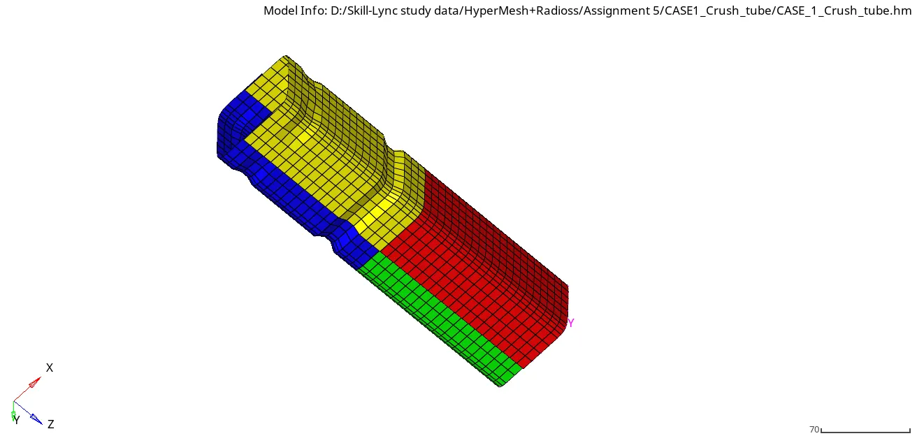
Apart from this model, one more important thing is the Property Card and Material Card set up.
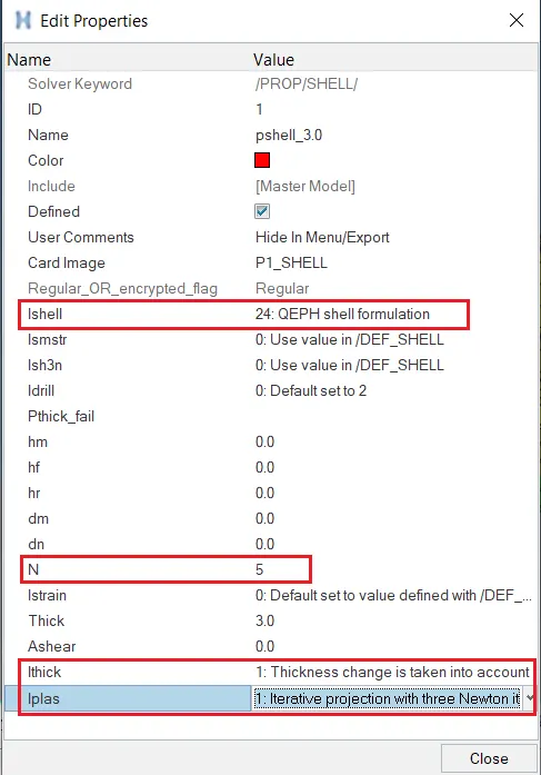
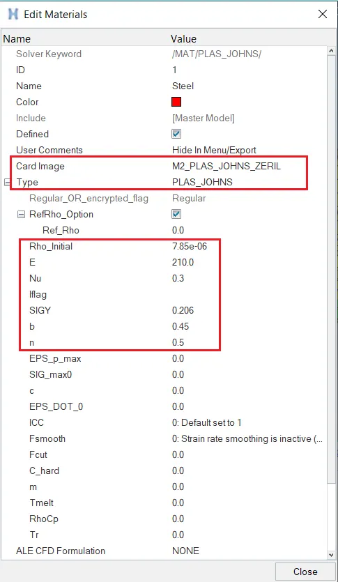
The first image is of a Property card and the second one is of Material Card which are pre-defined for this model. By going through them I find no need to change them for our case study. So from here on out over Property and material card remain the same during the entire study. (No failure johnson card introduced here )
CASE 1:-
-I had got one model named crash_tube in the ".rad" format with the instruction of RUN the file as it is.
-In the first case, we are gone RUN the model as it is without changing any set parameters. So to take a good look at the pre-defined parameter I had imported the file in "Hypercarsh" workbench. You can access it from the Hypermesh Menu bar --> Application--> Hypercrash.
-Either you can import the same ".rad " from the file manager or you can directly drag and drop inside the graphical area of the Hypercrash.
-After Importing the model into Hypercrash I had found out two pre-defined interfaces Typer 2 and Type 7 respectively.
-Initial Interface Type 7 and Type 2 setup is as follows,
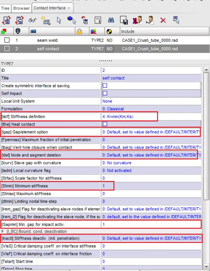
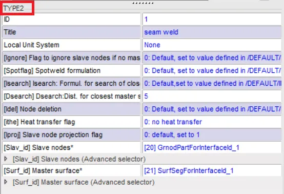
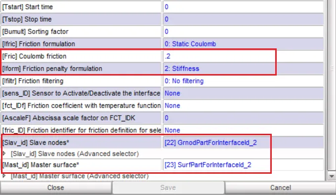
-AS you can see in the above images some of the parameters only changed to its recommended value all others are set to Default, which is not a good practice. We can also check and change these parameters from the Solver browser inside the Hypwermesh. But here you get a better explanation over each parameter.
After going through the interface types I had Exported the same ".rad" file and again open it to Hypermesh.
-After running the simulation you can observe the Data as follows,



-As you can understand from the above data Internal energy start to increase with a large amount at the start, In the intermediate section the rise in Internal energy is not that big (Difference very minimum) and as we reach at the end of the simulation it will become more constant. The same goes for Kinetic Energy but in the opposite way.
-This way the Equilibrium gets to maintained and as both the energies are trying to match each other.
-The Energy error I had got is fluctuating between -0.0 to -4.6 and in the end, we get a -3.8 energy Error. As per the standards of the simulation Energy error in between +5 to -15% is acceptable, so it is in the acceptable range. This 0.8% energy error indicates there is energy generated as we are using the QEPH element to avoid Hourglass formulation.
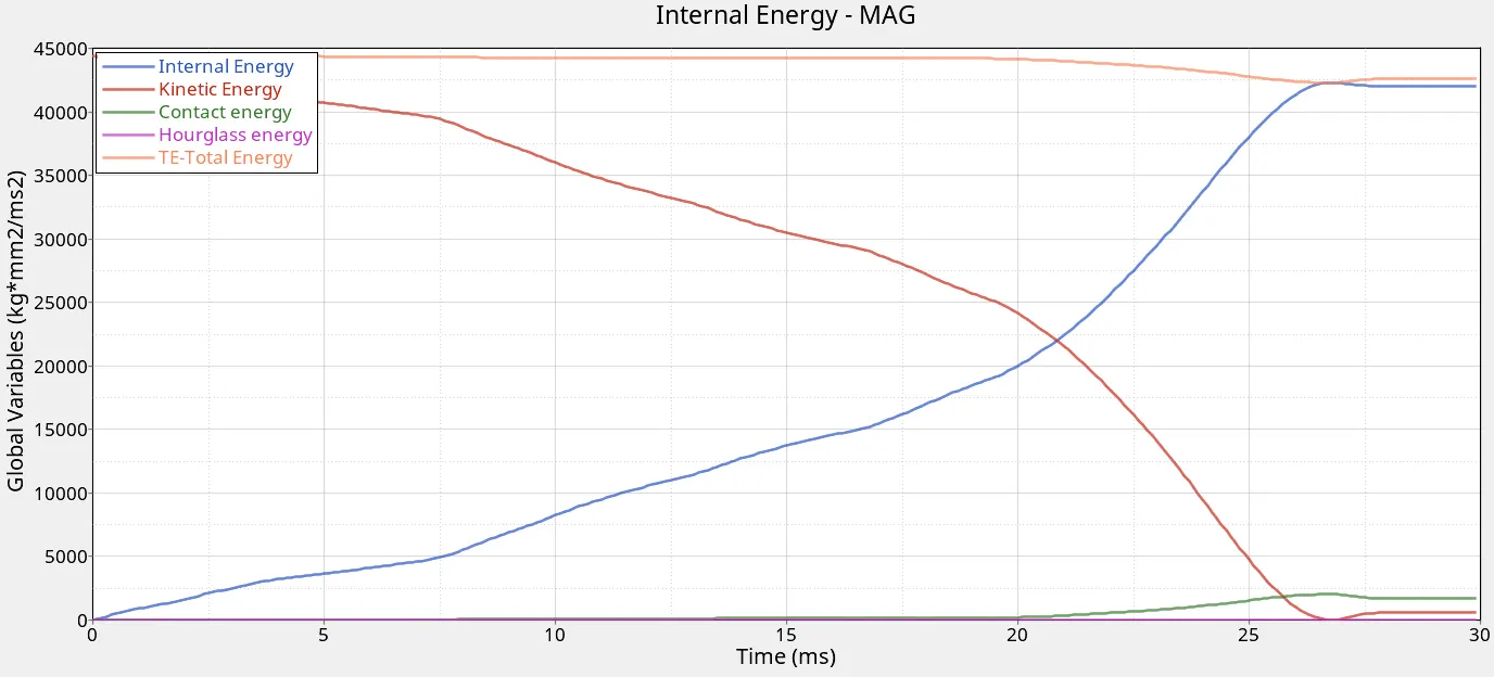
-Here you can see that the Internal Energy keeps on increasing and KE is decreasing with the same frequency. Contact energy is also increasing but the increase in contact energy is very minimum up until 15th ms and after 20th ms the contact energy stated raising. This is due to the surface get collapse badly up to this point there is self contact generated between the slave nodes and master surfaces.
-At the same 20th ms the Total energy starts to drop. After approximately 27th ms the KE is again starting to rise and IE starts to drop. This is because of the bounce effect we had experienced at the end of the simulation (In the last two frames of animation). This bounce is due to the High strain failure value is set to max there is no failure and the material behaves as an elastic one.
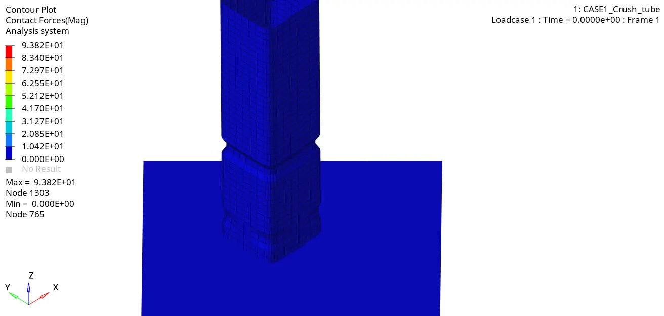
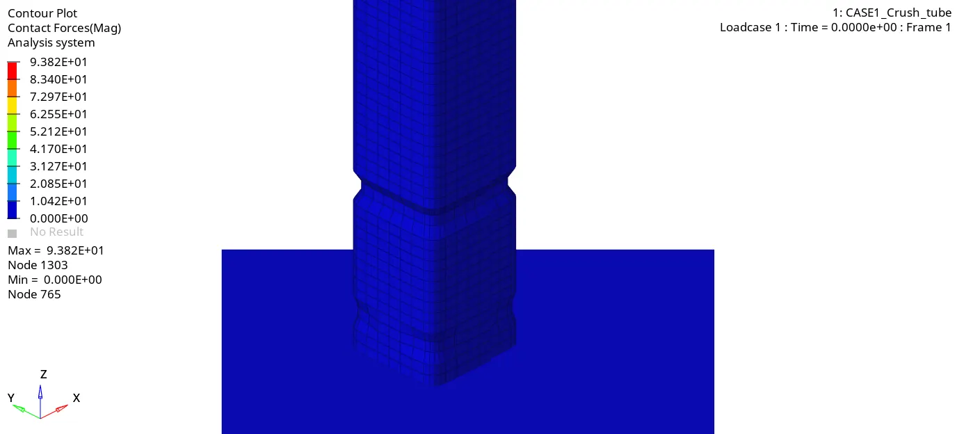
-You can also witness the contact force formulation at the end where a large amount of areas is in contact with each other. The Maximum contact force experience by this model is 93.8N.
CASE 2:-
-For Case 2, I had Specified the Inacti value to 6 and also did some other recommended parameter changes in the Type 7 Contact Card using Hypercrash workbench and then import this file in Hypermesh.
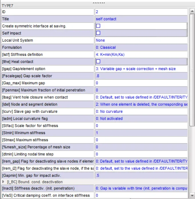
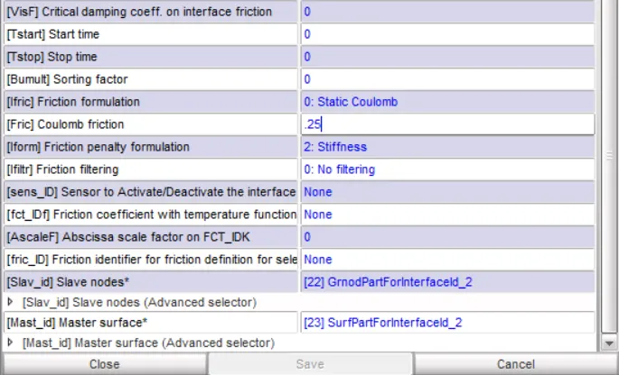
-After changing the recommended value I had RUN the simulation. After running the simulation I had got data as follows,



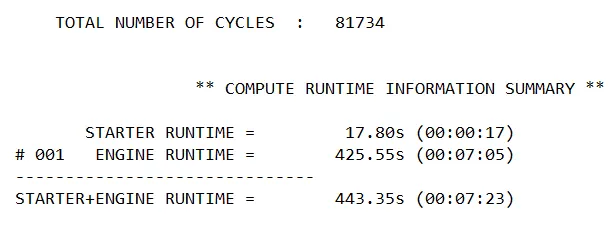
-As you can understand from the above data Internal energy starts to increase with a large amount at the start in the intermediate section the rise in Internal energy is not that big and as we reach at the end of the simulation it will become more stable. But the energy is kept fluctuating over time.
The same goes for Kinetic Energy but in the opposite way. This way the Equilibrium gets to maintain and both the as energies are trying to match each other.
-This way the Equilibrium gets to maintain and as both the energies are trying to match each other.
-The Energy error I had got is fluctuating between -0.0 to -5.7 and in the end, we get a -4.8 energy Error. As per the standards of the simulation Energy error in between +5 to -15% is acceptable, so it is in the acceptable range. This 0.8% energy error indicates there is energy generated as we are using the QEPH element to avoid Hourglass formulation.
-If you compare that with the CASE1 result the Energy error here is large also the KE in increase by a lot. Internal Energy is less as compare to the CASE 1 result. The least KE noted is 0.1364N and again increases due to the elastic nature of a material.
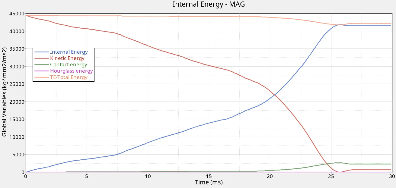
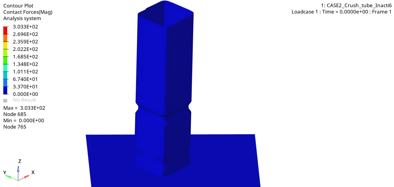
-Internal And Kinetic Energy behavior is the same as in CASE 1 but the Energy readings are different. contact energy rises just a little bit earlier as compare to the CASE1.
-At the very end of the simulation the model gets completely collapse which is the reason for the Contact Energy rise. Hourglass energy is zero the same as 1st case.
- Total energy starts to drop. After approximately 27th ms the KE is again starting to rise and IE starts to drop. This is because of the bounce effect we had experienced at the end of the simulation (In the last two frames of animation). This bounce is due to the High strain failure value is set to max there is no failure and the material behaves as an elastic one.
-You can also witness the contact force formulation at the end where a large amount of areas is in contact with each other. The Maximum contact force experience by this model is 303.3 N.
CASE:-3
- Under this CASE we are creating New interface which is Type 11. We are keeping the Type 7 contact intact. Type 11 is an edge to edge/ line to line contact.
-The parameters I had used during CASE 3 as follows,
-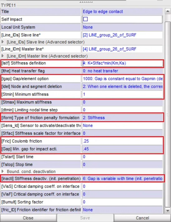
-Here you noticed the same parameters as we discuss in Type 7, so I had put the same recommended values here also.
-Now you are thinking about why I had set Igap values to the default one? The answer is I had already defined the Igap value in Type 7 contact properly and we are using both type 7 and type 11 interface in this simulation so we don't need to define the Igap value again. We can set it to default.
-I had also changed the value of Gapmin to 0.45 as per the instruction.
-As we have discussed earlier the Type 11 is for edge to edge contact.
After changing the recommended value I had RUN the simulation in hypermesh. After running the simulation I had got data as follows,



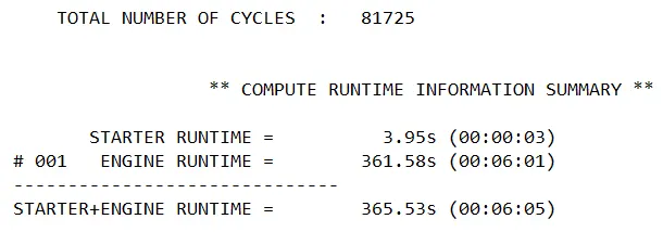
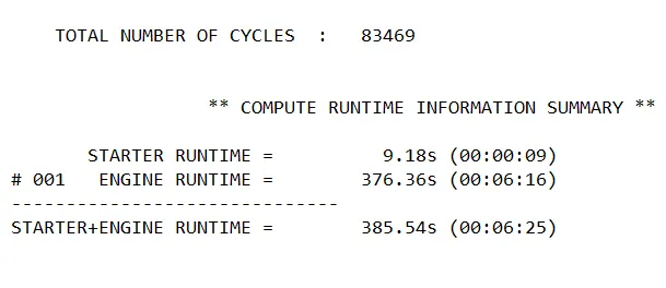
-Simulation time is less than the CASE 1 and CASE 2. also the number of cycles is also less.
- The energy error I had got was in between -0.0 to -5.7 %. Which is acceptable as per standards.
-We can notice the same energy behavior as we had noticed in CASE 2. The Minimum KE observed was 0.082 J after this it will again start to rise.
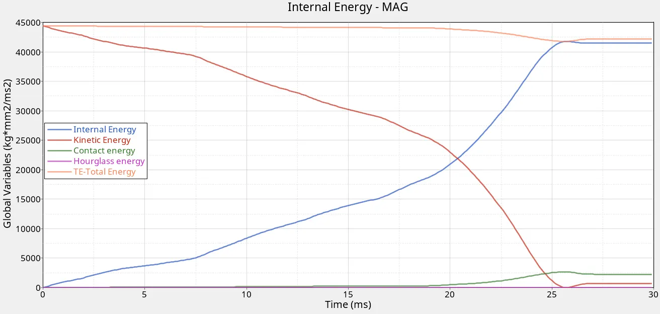
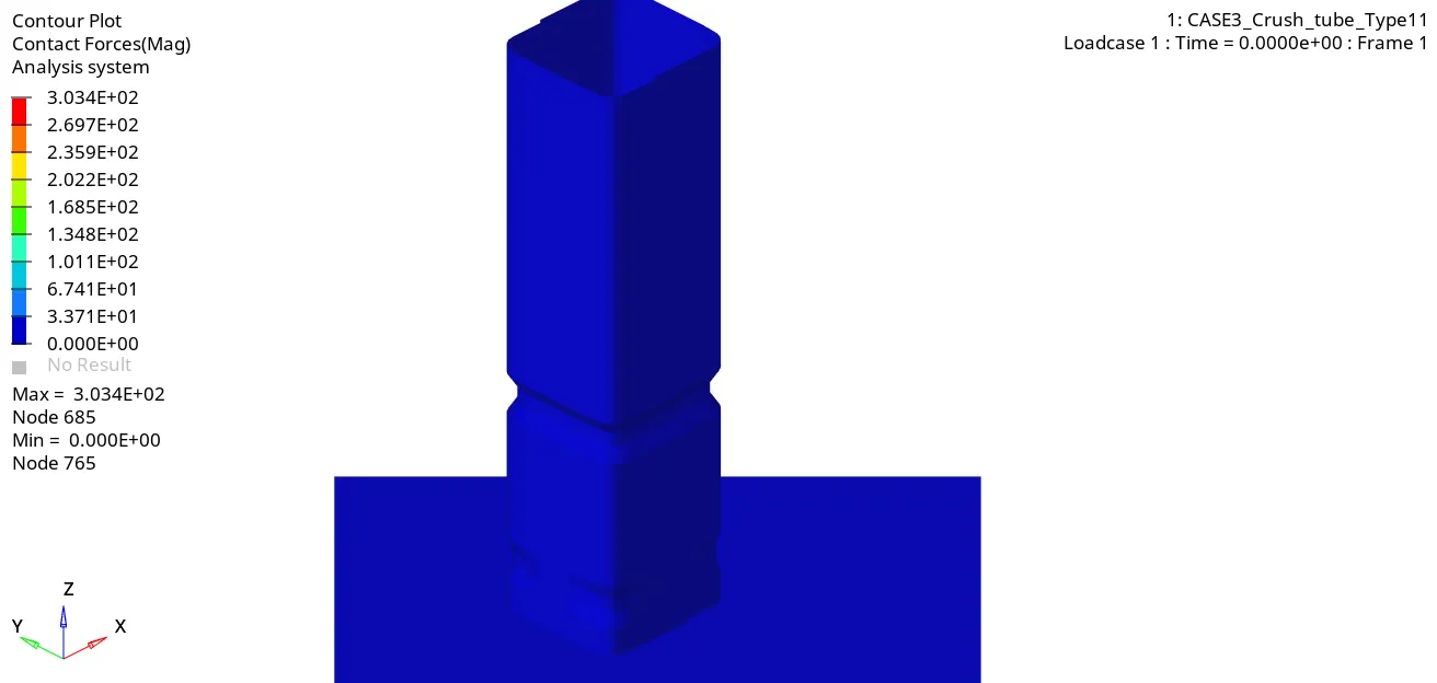
-The graphical behavior is almost the same as we observed in case 2. The maximum contact force is 303.4N. Which is the same as the result we are got from CASE2. Hourglass energy is zero through the simulation.
-At the very End the simulation the model gets completely collapse which is the reason for the Contact Energy rise.
OBSERVATION
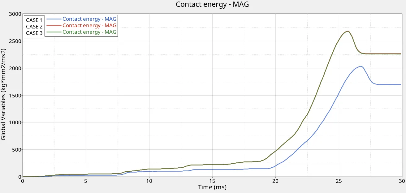
- The contact energy in the CASE of 2 and CASE 3 is higher than the 1st one. This is due to the Inacti and the other recommended values we provided during CASE 2 and 3. In 1st CASE we completely ignore the Initial Penetration and let the Default set values in the card to take care of it. Because of all these the contact energy is starting to rise a little bit late than CASE 2 and 3. Also, the amount of contact energy generated is very less and not showing the actual behavior of the model under the load.
-The Actual model Has two different thicknesses 2mm and 3mm respectively, and as per analytical calculation the default gap (physical gap) between the 2mm thickness component is 0.1mm and the, on the other hand, the 3mm components are penetrating each other at thickness level by 0.90 mm. So the model itself is not a good model.
-During 1st case where all values are set as default one (Igap=default), we set the GAPmin value =1mm, And if you went through the 1st segment of the report thoroughly where I specified this parameter conditions you will understand that the in this sort of situation Igap is considered as the value we are defined in GAPmin flag. Means the Radioss considered a 1mm gap for both the 2mm and 3mm thickness component and moved forward with the simulation. Because of this the contact energy recorded by the simulation is at the very end and very less as compare to CASE2 and CASE3.
-For CASE 2 and CASE 3 the parameters defined in there TYPE 7 Contact card is the same the only difference is we have added the TYPE 11 in the CASE3. But all the parameters inside the TYPE 11 contact interface is the same as the Type 7 7, Not much of a difference. Therefore we can witness approximately the same curve for both of these cases.
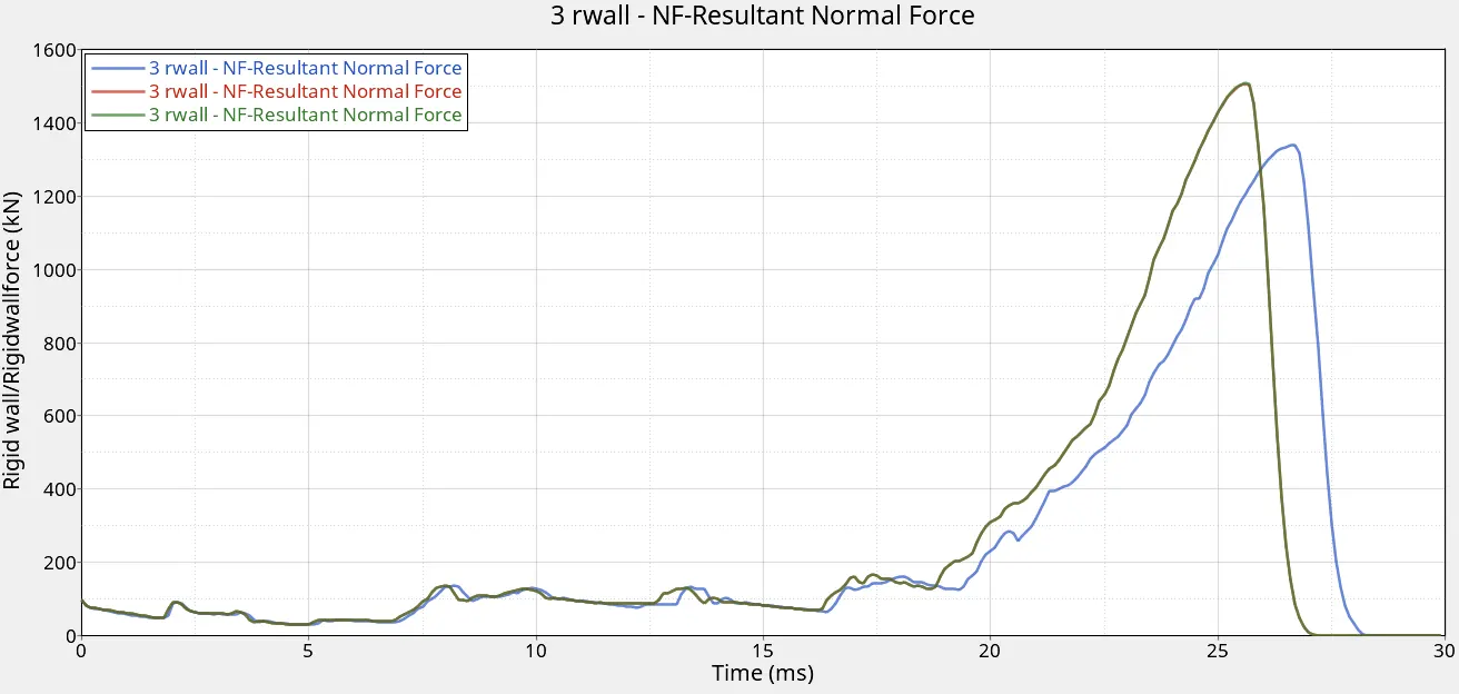
-As you can observe all these graphs the behavior of normal force through the simulation. The same behavior as we notice in the Contact Energy Development.
-The sudden drop at the very END is due to the elastic nature material/ model following. as at the very end of the simulation, you had noticed the minor bounce back, at that point in time Rigid body remove the forces on the model and as there are no forces on the body to push the model against the rigid wall you can find the drop in the graph.
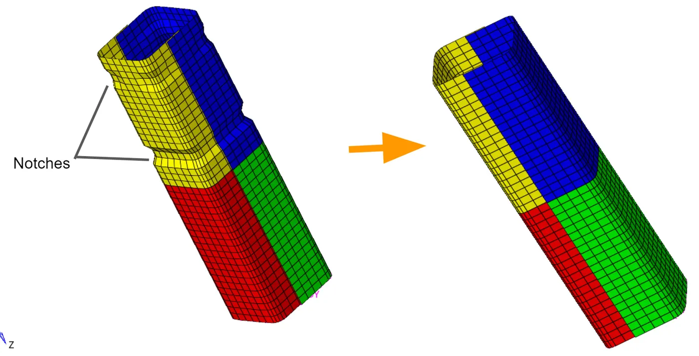
Effect of Notches on the model.
-I had set three new cases to study the effect of notches over the Model. As you can note in the previous case studies the model is starting to deform at the notches first therefore study of the notches is an important factor.
-For this study, we are following the same TYPE7 and TYPE 11 Interfaces which we are defined in CASE 3.
CASE4:-
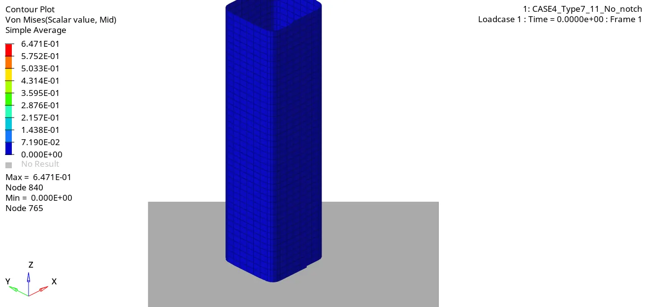
- We are Remove both notches and remove boundary conditions on the rigid body node and then RUN the model as it is.
-I had used the "Align Node" option from the Panel of Hypermesh to remove both of the Notches. (F7 is the shortcut key to accesses the option)
-Removing the Boundry condition means removing all degree of freedom restriction. so I had done the same.
-After removing the Boundry condition and notches I had RUN the simulation.


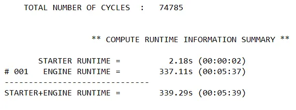
-The simulation Time we got is 5.39 and the numbers of cycles are 74785.
-The Energy created to avoid initial penetration is stored as an Energy error. the Energy error we got is in between -0.0 to -5.8.
-The initial Deformation happened at the point of contact over the Rigid wall. The first elements layer near the rigid wall experienced the resistance force first and deformed accordingly and from that point onward strain is starting to induced and transferred through the model.
CASE5:-
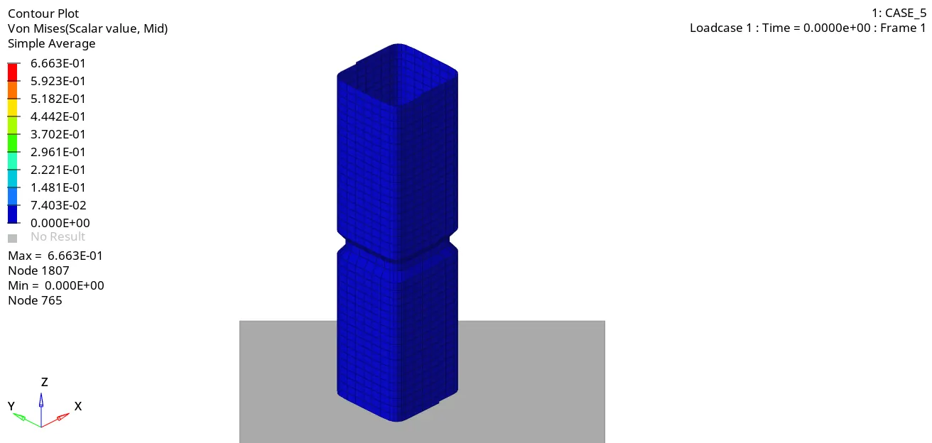
- In this case, We are creating a notch in the middle and add boundary conditions on the rigid body node and then RUN the model.
-I had used the "Translate" option from the Panel of Hypermesh to creat a Notch. (shift + F4 is the shortcut key to accesses the option)
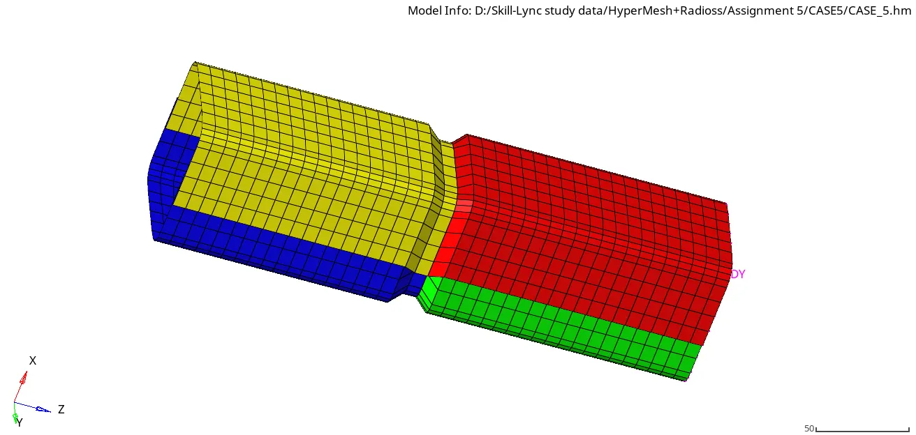
-After running the simulation the results I have got is was as follows,



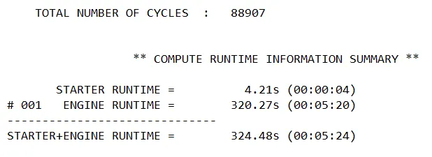
-The simulation Time we got is 5.24 and the numbers of cycles are 88907.
-The Energy created to avoid initial penetration is stored as an Energy error. the Energy error we got is between -0.0 to -7.00.
-The initial Deformation happened at the Notch. The first elements layer near the center notch experienced the resistance force first and deformed accordingly and from that point onward strain is starting to induced and transferred through the model.
CASE6:-
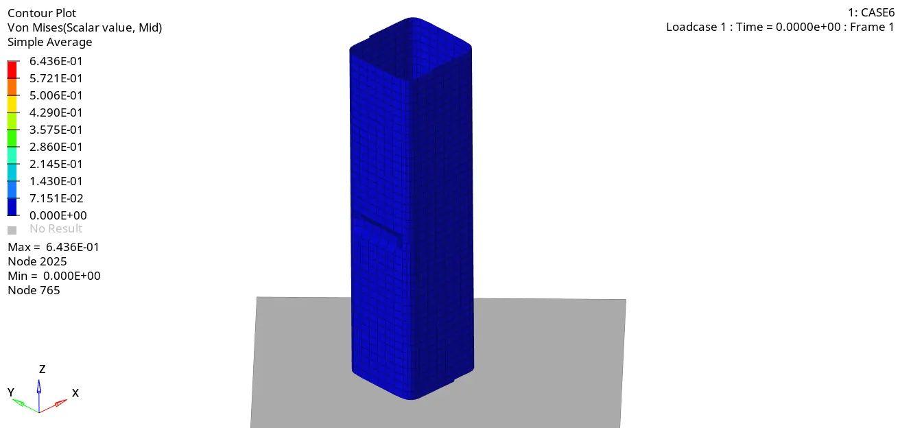
- In this case, We are creating a notch and add boundary conditions on the rigid body but the notch is on opposite faces of each other only. Not like we see in earlier cases.
-I had used the "Translate and Align node" options from the Panel of Hypermesh to creat a Notch. (shift + F4 & F7 is the shortcut key to accesses the option respectively)
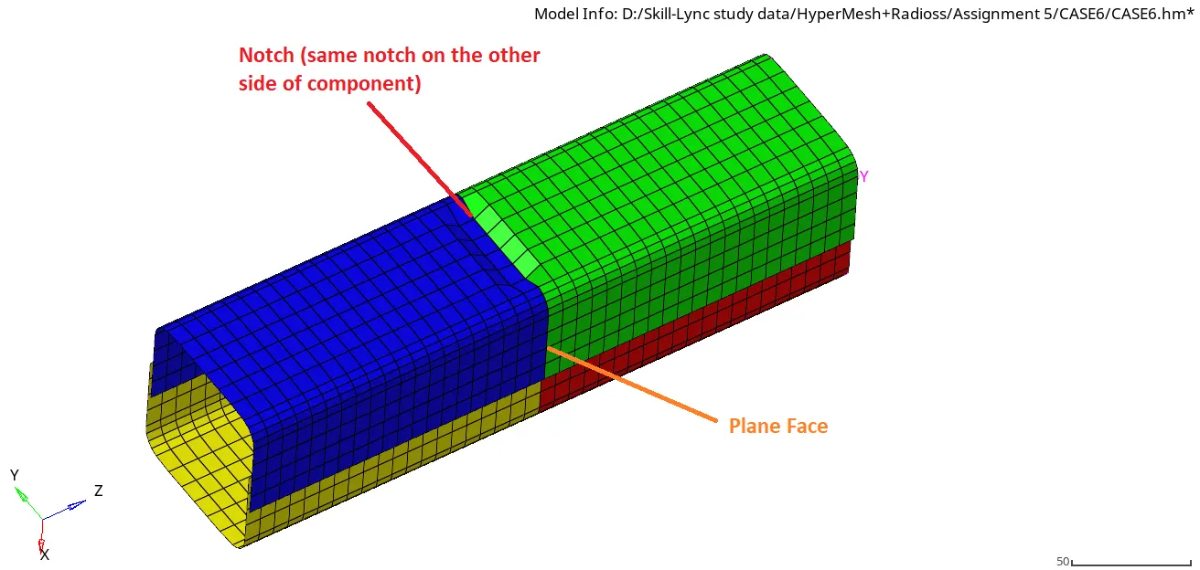
-After running the simulation the results I have got is was as follows,



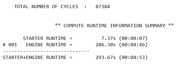
-The simulation Time we got is 4.53 which is less than the CASE4 and CASE5 for the numbers of cycles 87384.
-The Energy created to avoid initial penetration is stored as an Energy error. the Energy error we got is between -0.0 to -6.6.
-The initial Deformation happened at the Notch. The first elements layer near the center notch experienced the resistance force first and deformed accordingly and from that point onward strain is starting to induced and transferred through the model.
Observation
The animation results as follows for three cases, Here we are looking to Von Mises Stress which will give better stress translation over the model visually.
-After Studying all the cases I can say that the Notch making a very huge impact on energy absorption and deformation of the component.
-The model is starting to deformed at Notch first if there is any notch present. If not then the force is directly applied against the opposite end of the model which we can see in case 4.
-In CASE 4 the where No notch is present the model is getting compressed against the rigid wall and the face which is in contact with the rigid wall experience the force first. inside the model resistive force is generated to oppose the deformation. The force is not that much because there are no uneven Ups & downs (Notches) over the body. The notches create more resistance to the deformation hence more the force is need to apply to the element for deformation.
-In CASE 5 and CASE 6 deformation is started at the notch first.
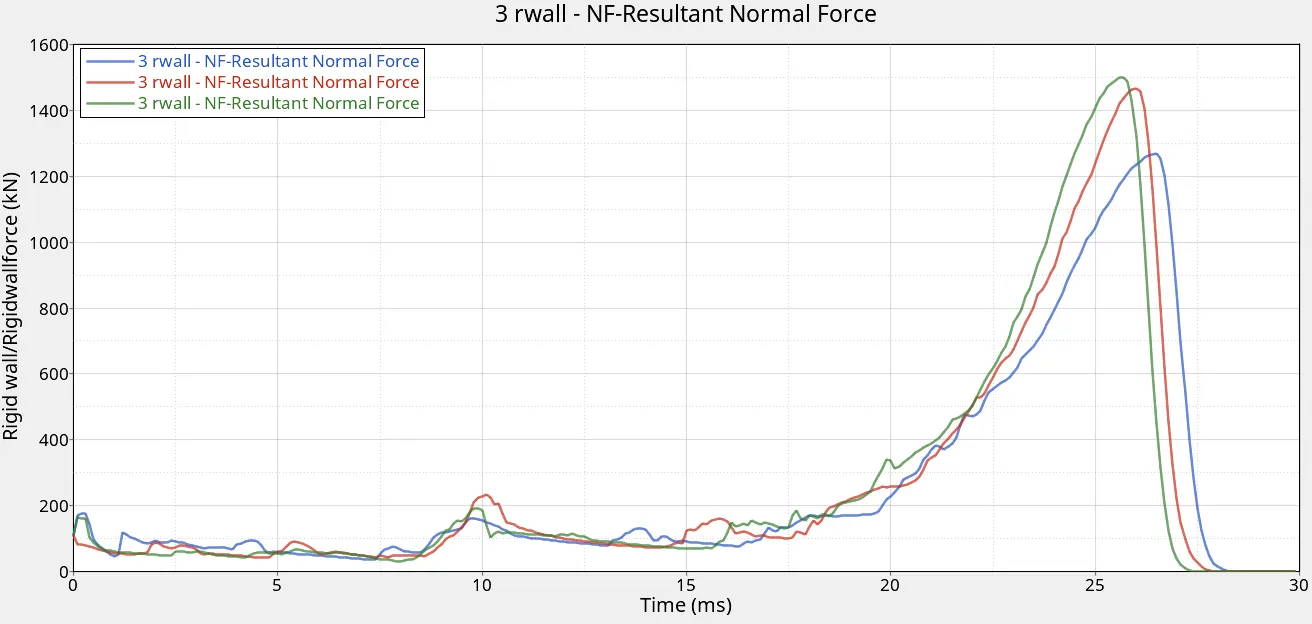
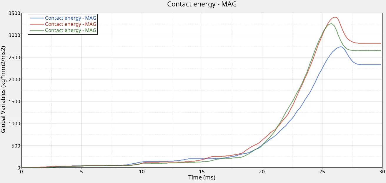
-The normal force graph and Contact energy graph are different from each other only due to the different sorts of Notch formations.
-For CASE 4 as we discuss earlier deformation takes place at completely opposite side of the force applied. Also, the contact forces are very less in this case because the deformation happens inside the model in linear nature, The Deformation happening element line by line.
-In case 5 and CASE 6 the notch is responsible for such high contact energy. In CASE 5 where the notch is in the middle and enveloped all four sides the high stress is generated, You can see that in the Animation results. Self impacting happen near that area after the element near the Notch gets completely collide the force is starting to move forward, This Notch is Breaking the model from the middle first. recorded high contact energy of all.
-In CASE 6 where Notch is in middle but only on the two opposite faces, recorded contact energy less than CASE 5 but more than CASE 4 and at the same time highest Normal force of all. This Extra developed force is due to the Notch representation over the model. As the Notch in CASE 6 has two opposite surfaces plane when the force in applied on the model it will impact the notch part first but the neighboring element of that notches having straight faces. To deformed that faces more force are getting applied which will result in high force values.
Conclusion:-
- Type 7 Interface is good for a node to surface as well as Self impact surfaces.
- The Type 7 interface along with Recommended parameters gives a more realistic result than its Default setup.
- Using Type 7 Interface with and without Type 11 interface will give the approximately the same result. But defining both is always a good practice.
- Different sorts of Notches over the different segments of the model will impact the simulation result for the same Interface setup.
-Notches create more resistance to the deformation.