Assignment 4-RADIOSS Material Laws Challenge
Aim -
- To run the simulation for the plate and rigid ball by using Jhonson Cook Material and Elasto Plastic Material by using Radioss solver. And compare the results for all cases.
Objective -
- To find out the total number of cycles, Energy Error, Mass Error, and Simulation Time.
- Run the simulation by changing the material, shell properties, and failure parameters.
- Run the simulation for all 7 cases.
- Run the simulation by converting the Failure Jhonson Model to LAW 1.
- Compare all the 7 cases results.
Introduction
Below shown some material properties continuously used while doing the material selection.
In the form of a material card
Law1-Elastic
Law2- Johnson cook
Law27- Elastic-plastic brittle
Law36- Elastic-plastic tabulated
Law42- Visco Hyperelastic
Law70- Foam
In the form of material properties
- Isotropic elasticity
- Isontropic elasto-plastic
- composites and anisotropic
- Viscous
- Hydrodynamics
- Explosives
Law 1 Elastic
- Isotropic means that a material will have the same properties in all directions.
- Under isotropic elasticity, Radioss provides 2 types of elasticity
- Linear Elasticity- Law1 elastic
- Hyperelastic - LAW 69 Tabulated hyperelastic
- The Radioss elasticity law follows the hooks law of elasticity so, there is a linear relationship between stress and strain.
- It is available for beam, Truss, shell, and solid elements.
- This material is exclusively for elastic materials.
- Material stiffness is determined by the modulus of elasticity. Poisson's ratio and shear modulus are calculated.
- G=E/2(1+`nu`)
Law2 Johnson-cook material(PLAST_JOHNS)
- 1) It's also called as plast_john material model.
- 2) This model calculates the stress using plastic strain this stain rate and temp change.
- 3) So, in case doing multiple analysis case with higher deformation to induce the plastic strain then those things are ideal material models.
- 4) This model expressed material stress as a function of strain, strain rate, and temperature.
- 5) A build-in-failure criterion based on the maximum plastic strain is available.
Law 36 Elastic-plastic
- This law model an isotropic elastoplastic material using user-defined functions for the work hardening portion of the stress-strain curve for the different strain rates.
- Isontropic elasto plastic material.
- user-defined function for the work for the hardening portion of the stress-strain curve. it is also available for brick and shell materials.
- The elastic portion of the material stress-strain curve has been defined by the youngs modulus and Poisson's ratio.
- Material plasticity curves can be given for an arbitrary number of strain rates.
- Linear interpolation of strain stress curve.
Law27 (PLAST BRIT)Elastoplastic material with brittle failure
- This law is combined an isotropic elastoplastic johnson cook material model with an orthotropic brittle failure model. Material damage is accounted for prior to failure.
- Failure and damage occur only in tension. This law is applicable only for shells.
- Yield surface definition same as johnson cook
- Damage and rupture are defined with 4 parameters for each principal direction.
As similarly there are given below
Law 42 - Hyperelastic behavior
- This is mainly the hyperelastic behavior(nonlinear elastic)
- This law is generally used to model polymers and elastomers
Law70 - Tabulated foam
- This law is of Viscoelastic behavior in the materials.
- The stress and strain relationship is defined by functions according to strain rate.
- Unloading behavior is defined by curves and hysteresis parameters.
Procedure
To know these all the laws to perform the different material properties with the post-processing the results.
Case1: Run the model as it is. Name it as law2_epsmax_failure.
Import the model from the solver deck as the johnson _0000.rad. Click on import.
As per case 1, the material has been shown. Keep the material card as it is.
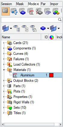
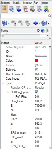
Run the given model as it is and name it Law2_epsmax_failure.

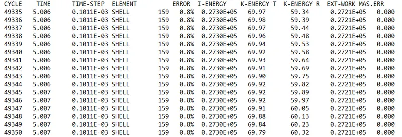
After running the case1 file the analysis has been saved. After opening 0001.out file.

splitting the screen into the required numbers as shown below.

Run the animation file in the hyperview.
The h3d file has been imported and applied.

The animation file has been run in the contour, the result type is to be in von mises and apply.
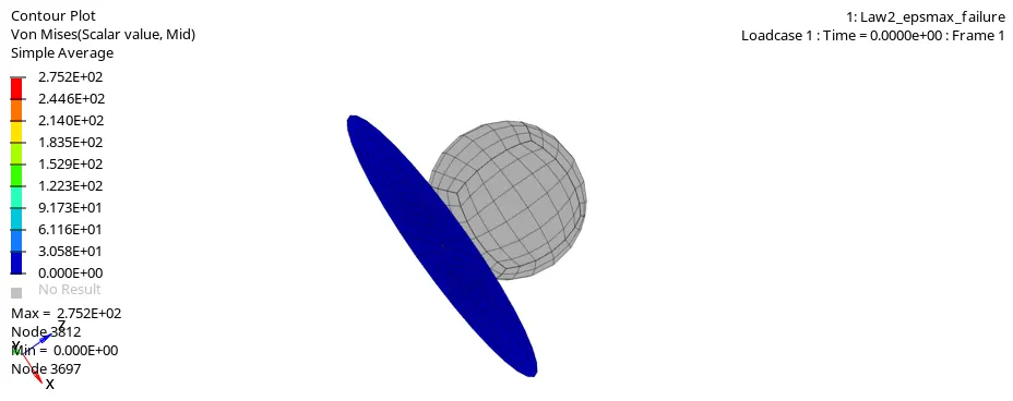
The animation image has been shown below. By visualizing the animation image the elements get deleted before its reaches the max. limit.
Plot the graph for all energies by using the hypergraph
Import the TO1 file by selecting the global variables with different types of energies and apply.
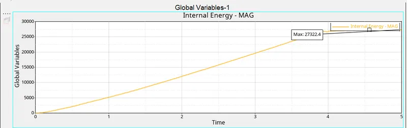
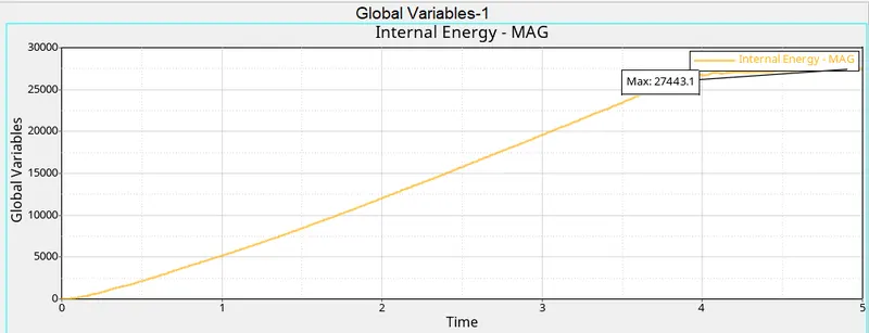
All energies can be discussed separately. below shown the internal energy graph.
To verify the max note in the graph will be taken by selecting the single curve math.
As we concluded the internal energy has been starting from the origin, there are not having any changes in the material as initially.
After by time interval rigid body hits the object(plate) and the graph goes on increasing. It has been the constant for some time interval.
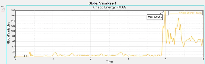
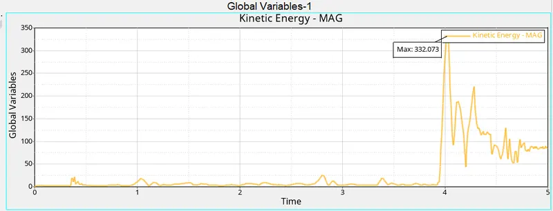
For kinetic energy graph was initially low for the base plate. It shows some variations in the graph due to sound waves. Once hitting the rigid body into the deformable object it has been increasing as shown below and the max point has been reached.
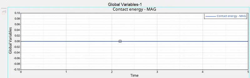
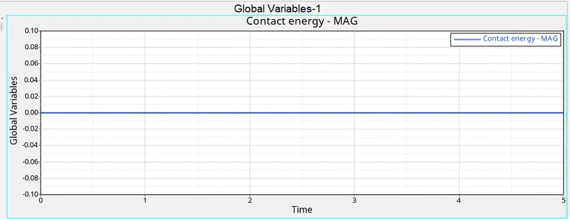
The contact energy is constant in the graph because there are two different types of materials of rigid body and base plate.
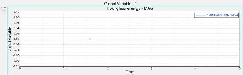
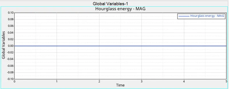
Due to the standard parameters assigned, the hourglass effect has been constant and shown in the figure.
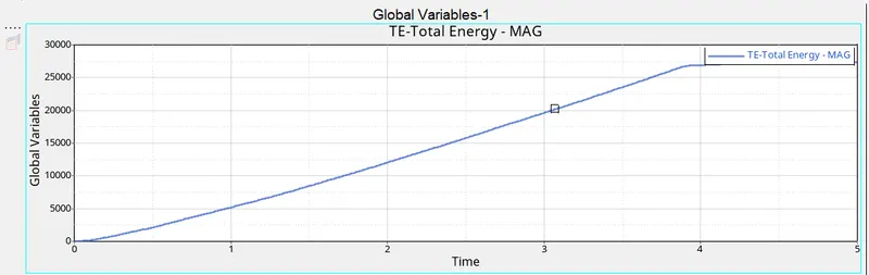
Total energy has been taken into account of all resultant energies and it has been starting from where the energy error will occur. The energy error will be in the range of -15% to 5% is acceptable. Particularly for this case, the energy error has been shown as 0.8% so, it is acceptable.
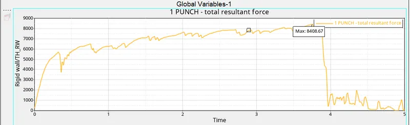
The rigid body force can also be plotted in the graph as a rigid wall, total resultant forces, and apply.
The below fig has shown the total resultant force for the rigid body that has been starting from the origin and before hitting the rigid body to the deformable base plate. The resultant force will increase after some time interval once hitting the base plate the force will be reduced. It’s shown in the graph.
Following are the result got from case 1.
Total number of cycles = 49379
Energy error = 0.8%
Mass error = 0%
Simulation time = 524.55 s
Case2 : In/FAIL/JOHNSON,change ifail_SH=1,Dadv=1 and lxfem=1. Run the model as Law2_epsmax_crack.
Assigning the given parameters to FAIL/JOHNSON
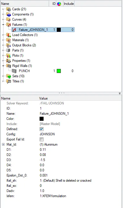
Run the model and name it Law2_epmax_crack.

Open the 0001.out file. It shows all results for the energies.
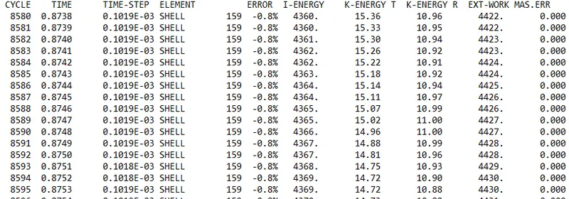

The h3d file has been imported and applied.

The animation image has been shown below.
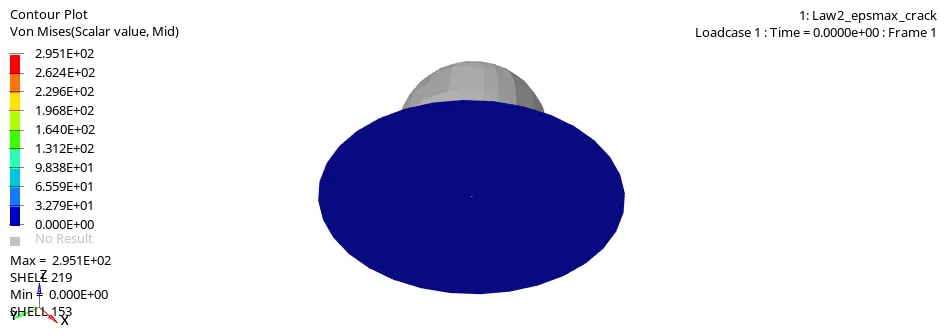
Import the T01 file and plot the graphs.
In internal energy, it has been starting from the origin and gradually increases w.r. t time period. Initially, there is no variation in the deformation. After some time interval, the deformation will occur in the base plate.
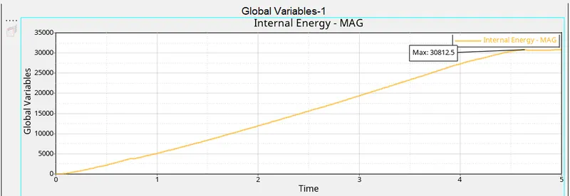
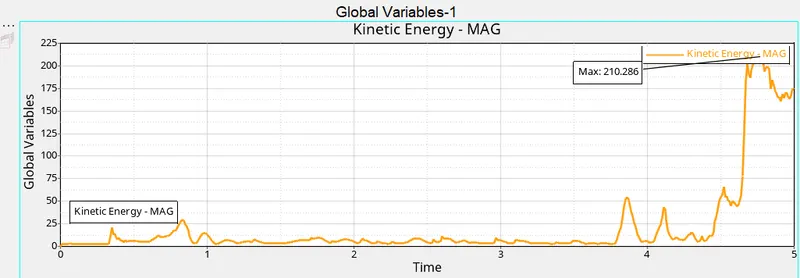
The K.E of the deformable base plate is constant but some variation will occur because of the speed of sound after hitting the rigid body to the base plate. K.E will increase until the base plate gets cracked.
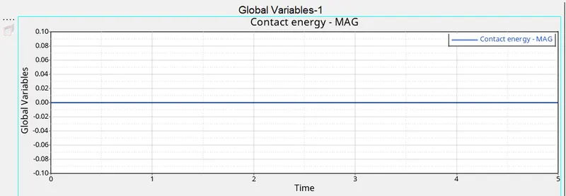
The contact energy will be constant over the simulation because 2 different surfaces of material get into contact.
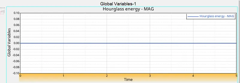
Hourglass parameters are assigned, so it will be constant.
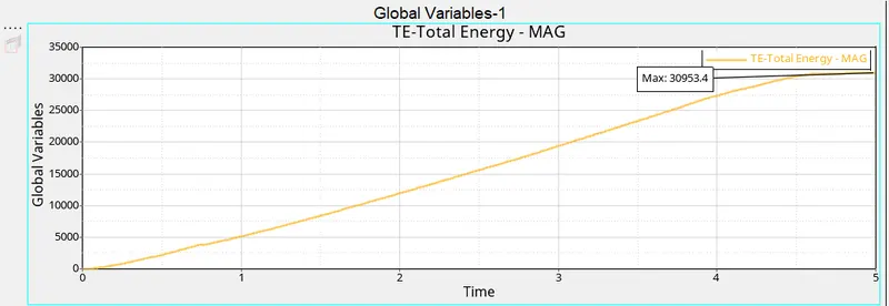
Total energy has been taken into account of all resultant energies and it has been starting from where the energy error will occur. The energy error will be in the range of -15% to 5% is acceptable. Particularly for this case, the energy error has been shown as 4.1% so, it is acceptable.
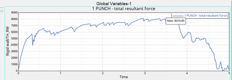
The total resultant forces have been starting from the origin and due to K.E, the total resultant forces are high. when it hit the base plate it will start decreasing as shown below.
Following are the result got from case 2.
Total number of cycles = 49217
Energy error = 4.1%
Mass error = 0%
Simulation time = 624.32 s
Case3: Delete the /FAIL/JOHNSON card, Run the model as Law2_epsmax_nofail.
For this case delete the failure johnson material model. Run the given model and name it Law2_epmax_nofail.

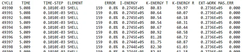
Open the 0001.out file. It shows all results for the energies.

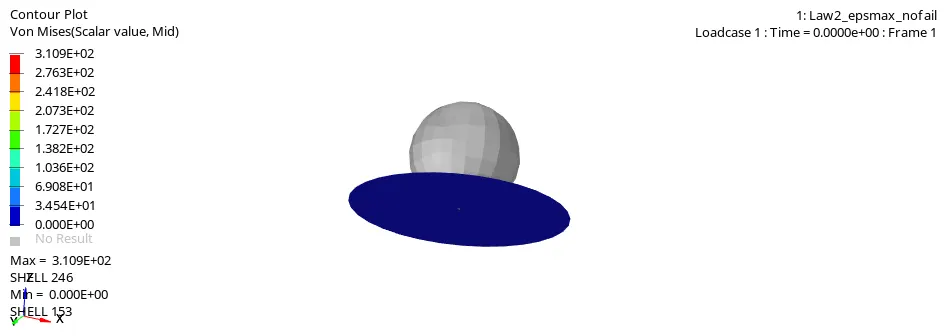
The h3d file has been imported and applied.

The animation image has been shown below.
Import the T01 file and plot the graphs.
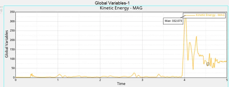
For this case initially, there is no deformation occurring in the base plate, so the graph is starting from the origin.
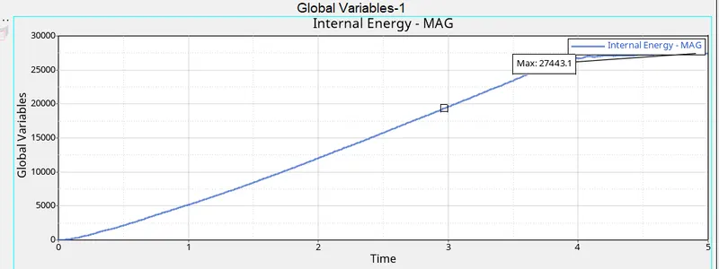
The kinetic energy has not been applied to the base plate when the rigid body comes in contact with the base plate.
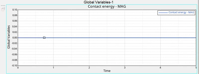
The contact energy will be constant over the simulation because 2 different surfaces of material get into contact.
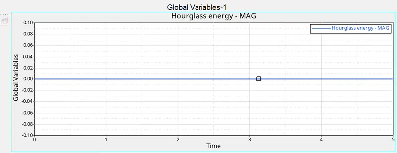
Hourglass parameters are assigned, so it will be constant.
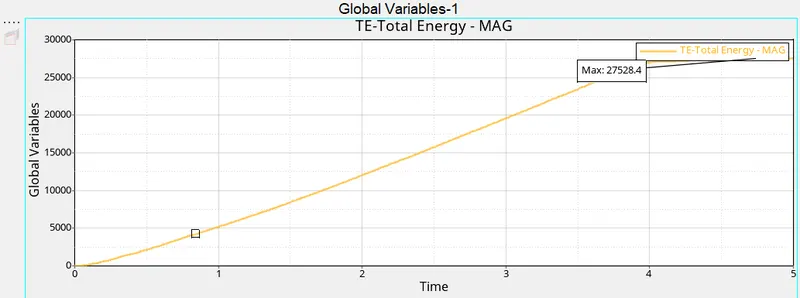
Total energy has been taken into account of all resultant energies and it has been starting from where the energy error will occur. The energy error will be in the range of -15% to 5% is acceptable. Particularly for this case, the energy error has been shown as 0.8% so, it is acceptable.
For the rigid wall, forces have been initially increasing and after some time rigid body hit the deformable base plate and the forces start to decrease and it's shown below.
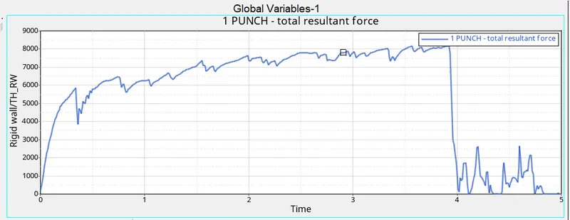
Following are the result got from case 3.
Total number of cycles = 49408
Energy error = 0.8%
Mass error = 0%
Simulation time = 502.65 s
Case4: Delete the value of EPS_p_max and run the model with the name Law2.
For this case delete EPS_p_max the failure johnson material model. Run the given model and name it Law2.
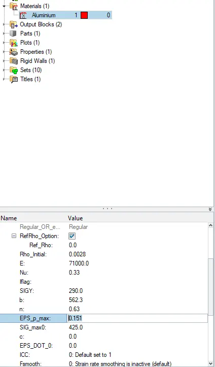

Open the 0001.out file. It shows all results for the energies.

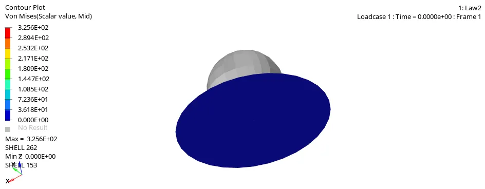
The h3d file has been imported and applied.

The animation image has been shown below.
Import the T01 file and plot the graphs.
For this case initially, there is no deformation occurring in the base plate, so the graph is starting from the origin.
The kinetic energy has not been applied to the base plate when the rigid body comes in contact with the base plate.
The contact energy will be constant over the simulation because 2 different surfaces of material get into contact.
Hourglass parameters are assigned, so it will be constant.
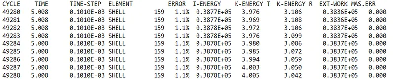
Total energy has been taken into account of all resultant energies and it has been starting from where the energy error will occur. The energy error will be in the range of -15% to 5% is acceptable. Particularly for this case, the energy error has been shown as 1.1% so, it is acceptable.
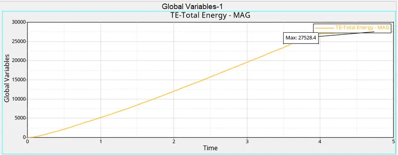
The rigid wall forces start from the origin and go on increasing gradually.
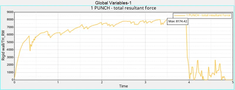
Following are the result got from case 4.
Total number of cycles = 49304
Energy error = 1.1%
Mass error = 0%
Simulation time = 624.79 s
Case 5: Convert this material model to Law1 elastic with the same density, E, nu and run.
As per case 5, select the material card as M1_ELAST.
other parameters keep as it is.
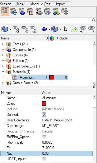
Run the given model and name it Law1.

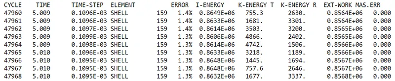
Open the 0001.out file. It shows all results for the energies.
The h3d file has been imported and applied.

The animation image has been shown below.
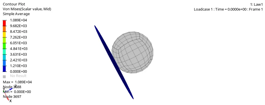
Import the T01 file and plot the graphs.
For this case initially, there is no deformation occurring in the base plate, so the graph is starting from the origin.
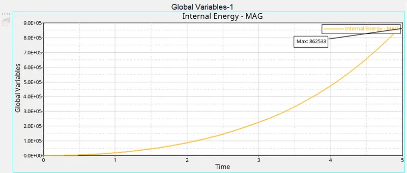
The kinetic energy has not been applied to the base plate when the rigid body comes in contact with the base plate.
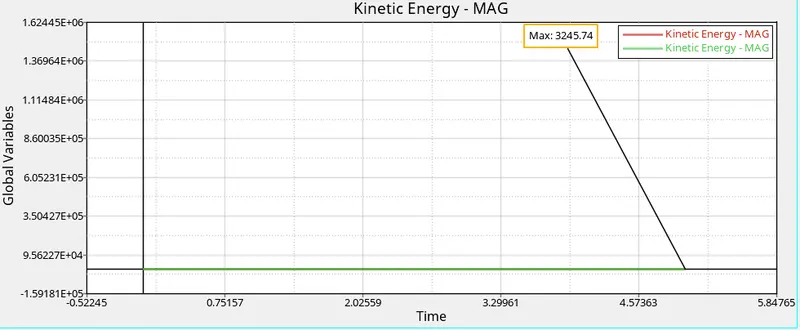
The contact energy will be constant over the simulation because 2 different surfaces of material get into contact.
Hourglass parameters are assigned, so it will be constant.
Total energy has been taken into account of all resultant energies and it has been starting from where the energy error will occur. The energy error will be in the range of -15% to 5% is acceptable. Particularly for this case, the energy error has been shown as 1.3% so, it is acceptable.
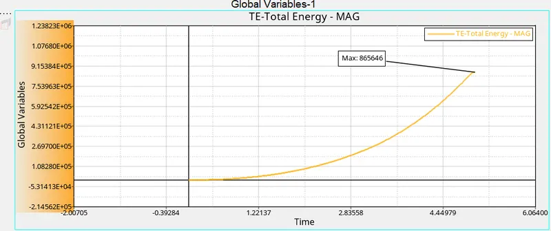
The rigid wall forces start from the origin and go on increasing gradually.
Following are the result got from case 5.
Total number of cycles = 47969
Energy error = 1.3%
Mass error = 0%
Simulation time = 547.82 s
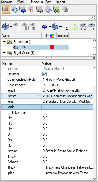
Case 6: Open the Law27_0000.rad. Change the shell properties as the recommended shell properties.
For this case import the law27 model. Run the given model by changing its shell properties to recommended values.

Open the 0001.out file. It shows all results for the energies.

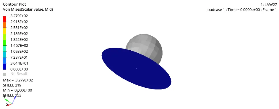
The h3d file has been imported and applied.

The animation image has been shown below.
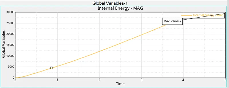
Import the T01 file and plot the graphs.
For this case initially, there is no deformation occurring in the base plate, so the graph is starting from the origin.
The kinetic energy has not been applied to the base plate when the rigid body comes in contact with the base plate.
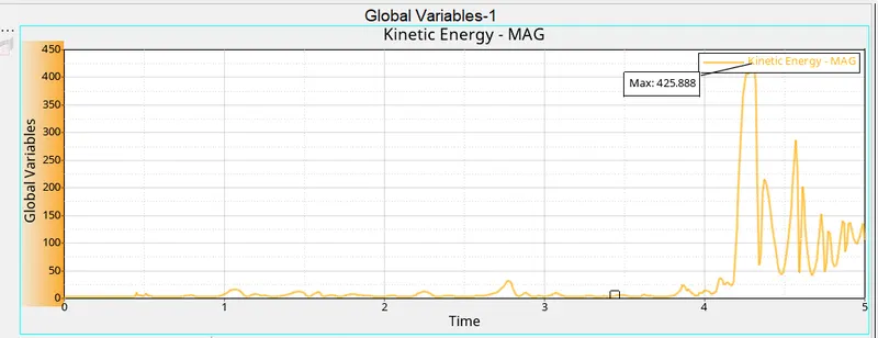
The contact energy will be constant over the simulation because 2 different surfaces of material get into contact.
Hourglass parameters are assigned, so it will be constant.
Total energy has been taken into account of all resultant energies and it has been starting from where the energy error will occur. The energy error will be in the range of -15% to 5% is acceptable. Particularly for this case, the energy error has been shown as 0.8% so, it is acceptable.
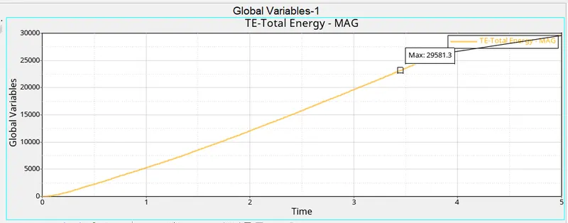
The rigid wall forces start from the origin and go on increasing gradually.
Following are the result got from case 6.
Total number of cycles = 49508
Energy error = 0.8%
Mass error = 0%
Simulation time = 593.03 s
Case 7: Convert the card to a Law36 elastoplastic tabulated.
Import the model from the solver deck as the johnson _0000.rad. Click on import. Change its shell properties to recommended values.
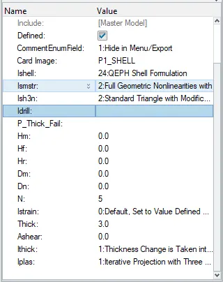
First, create a new curve.
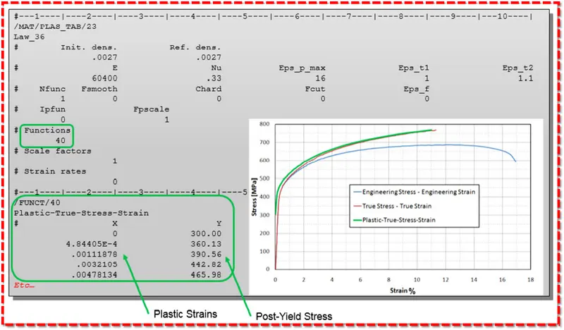
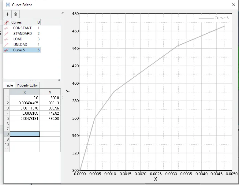
Assign the given values to the curve.
Select the M36_PLAST_TAB card.
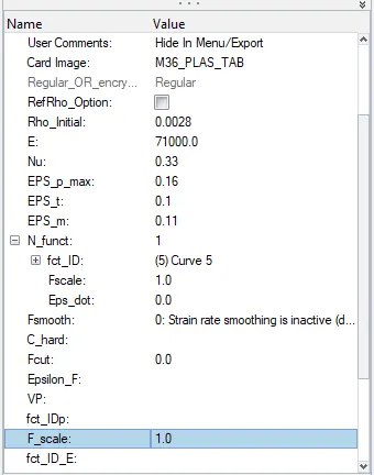
After assigning all the parameters run the rad file and save it as Law36.

Open the 0001.out file. It shows all results for the energies.
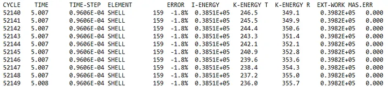

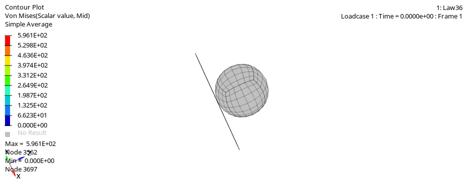
The h3d file has been imported and applied.

The animation image has been shown below.
Import the T01 file and plot the graphs.
For this case initially, there is no deformation occurring in the base plate, so the graph is starting from the origin. As it is elastoplastic material it should resist the deformation till the yield point and after that base plate should break.
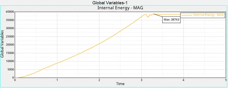
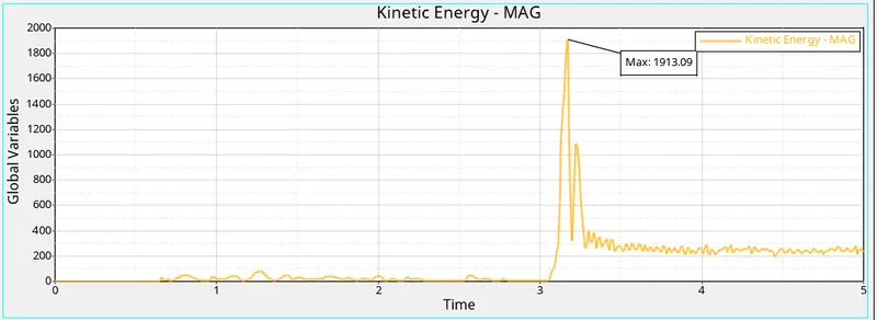
Initially, the K.E. is zero. After some time when the rigid body comes in contact with the base plate, it starts increasing.
The contact energy will be constant over the simulation because 2 different surfaces of material get into contact.
Hourglass parameters are assigned, so it will be constant.
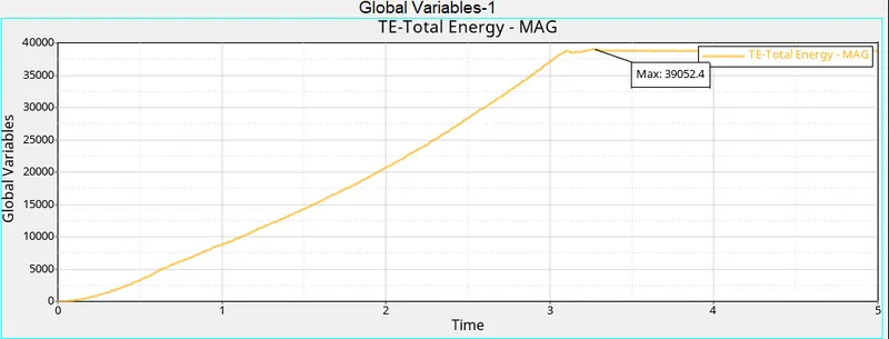
Total energy has been taken into account of all resultant energies and it has been starting from where the energy error will occur. The energy error will be in the range of -15% to 5% is acceptable. Particularly for this case, the energy error has been shown as -1.8% so, it is acceptable.
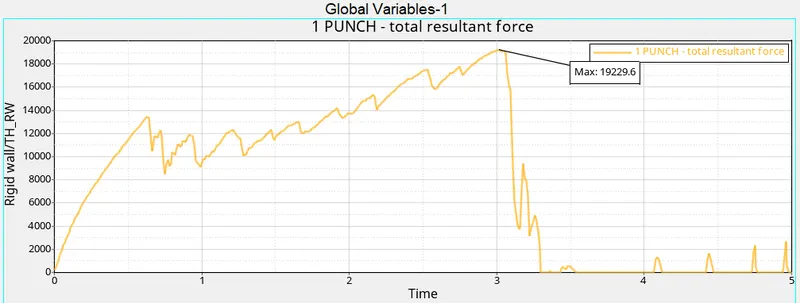
Initially, the rigid wall force will start from the origin and increase with some instant. After some time the resultant force will start to decrease.
Following are the result got from case 7.
Total number of cycles = 52176
Energy error = -1.8%
Mass error = 0%
Simulation time = 605.55 s
Comparison of results for all 7 cases
| Cases | Total Number of Cycles |
Energy Error (%) |
Mass Error (%) |
Simulation Time (S) |
Element Condition |
| Case 1 | 49379 | 0.8 | 0 | 524.55 | Elements deleted. |
| Case 2 | 49217 | 4.1 | 0 | 624.32 | Elements will be cracked and deleted. |
| Case 3 | 49408 | 0.8 | 0 | 502.65 | Elements deleted. |
| Case 4 | 49304 | 1.1 | 0 | 624.79 | Elements deformed, cracked but not deleted. |
| Case 5 | 47969 | 1.3 | 0 | 547.82 | Elements deformed, cracked but not deleted. |
| Case 6 | 49508 | 0.8 | 0 | 593.03 | Elements deleted. |
| Case 7 | 52176 | -1.8 | 0 | 605.55 | Elements deleted. |
Conclusion:
By observing all the results, we can say that Law36 is the best suitable material card. Because it shows both the behaviors of material i.e. Elasticity and plasticity. Because of this Law36 is widely used in companies.