Assignment 4-RADIOSS Material Laws Challenge

ASSIGNMENT 4 - RADIOSS Material Laws Challenge

Aim:

To apply different material types to the simulation model and compare the behaviour of the material with different element and failure formulations.

Objective:

To carry out simulations of the given starter files and compare the results. There shall be 7 cases (according to given parameters) and they are to be compared primarily via animations and plots. The files to be worked on are the FAILURE_JOHNSON_0000.rad file and the LAW27_0000.rad file. The cases are as follows:

• Law 2 (file: FAILURE_JOHNSON_0000.rad) - base simulation.
• Law 2 (file: FAILURE_JOHNSON_0000.rad) with Ifail_sh = 1, Dadv = 1, and Ixfem = 1.
• Law 2 (file: starter file for case 2) with fail/JOHNSON card deleted.
• Law 2 (file: starter file for case 3) with EPS_p_max value deleted
• Law 1 (file: FAILURE_JOHNSON_0000.rad) with fail/JOHNSON card deleted and values for density, E, nu assigned
• Law 27 (file: LAW27_0000.rad) with recommended shell properties
• Law 36 (file: LAW27_0000.rad) with recommended shell properties and given reference curve.

Theory:

• The accuracy of the simulation depends on the material chosen.
• Choosing the right material and providing the reliable material data in performing a simulation is very important.
• RADIOSS has multiple material properties and wide variety of material library like concrete, foam, rubber, composites etc.,
• Some of the commercially used material laws are:

Isotropic Elasticity - Law 1

• Isotropic means that a material will have the same material properties in all 3 directions. Under isotropic elasticity, RADIOSS provides two types of elasticity.
• Linear elastic: LAW1 elastic
• Hyperelastic: LAW69 Tabulated hyperelastic, LAW82 Ogden
• The RADIOSS elasticity law follows the hook’s law of elasticity i.e a linear relationship between the stress and starin.
• It is available for truss, beam, shell, and solid elements.
• As mentioned earlier, it is exclusively for elastic materials.
• The material stiffness is determined by Young’s modules of elasticity (E) and Poisson’s ratio (n).
• The sheer modulus G is calculated by

G=E2(1+V)�=�2(1+�)

Limitations:

• Elastic materials cannot be used for large deformation cases such as blow molding etc.,
• In the case of large deformation, law 2 johnson-cook material with high yield can be used.

Isotropic Elasto-Plastic

• RADIOSS provides various types of elasto-plastic material laws. It has all the material models based on von mises hardening without damage, von mises hardening with ductile damage, von mises with visco-plastic flow.
• Here, we are going to look at Johnson-cook/JOHNS and tabulated piece-wise linear/PLAS_TAB.

(PLAS_JOHNS) Johnson-cook material- Law 2

• This law represents an isotropic elasto-plastic material using the johnson-cook material model.
• The model expresses material stress as a function of strain, strain rate, and temperature.
• In the material card, we have an option called EPS_max which is nothing but plastic strain at failure. Failure of the element happens when 1 integration point reaches EPS_max.
• Now if failure is only based on EPS_max, there can be instances where the EPS_max gives out unrealistic results. To avoid this, we have the option called /FAILS/JOHN.
• /FAIL/JOHN card provides the user with more control over the failure of the johnson-cook strain.

LAW36-PLAS_TAB Elastic plastic piecewise linear material

• The LAW36 material law helps in modelling isotropic elasto-plastic material using user defined functions for the work hardening portion of the stress-strain curve for different strain rates.
• The curve defined is nothing but the stress-strain curve after the yield point. The yield point is set to 0.
• This material law is available for both brick and shell elements.
• If the work hardening portion is defined by the user, then its elastic portion is taken from the inputted young’s modulus and poisson’s ratio.
• Any number of stress-strain curves can be defined.
• The important part is that the strain rate curves must not intersect with each other.
• The plastic strain curve should start with 0.
• The user also has option to input yield stress with respect to pressure using fct_Idp.

PROCEDURE:

CASE 1:

Import the provided 0000.rad file into the HyperMesh workspace and change the properties to the recommended properties for shell elements.

Save the model and run the simulation without changing the failure card.

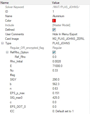
Material and failure cards for the simulation.

Below images show run and out file:-

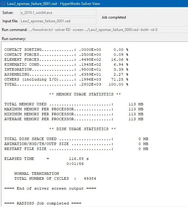
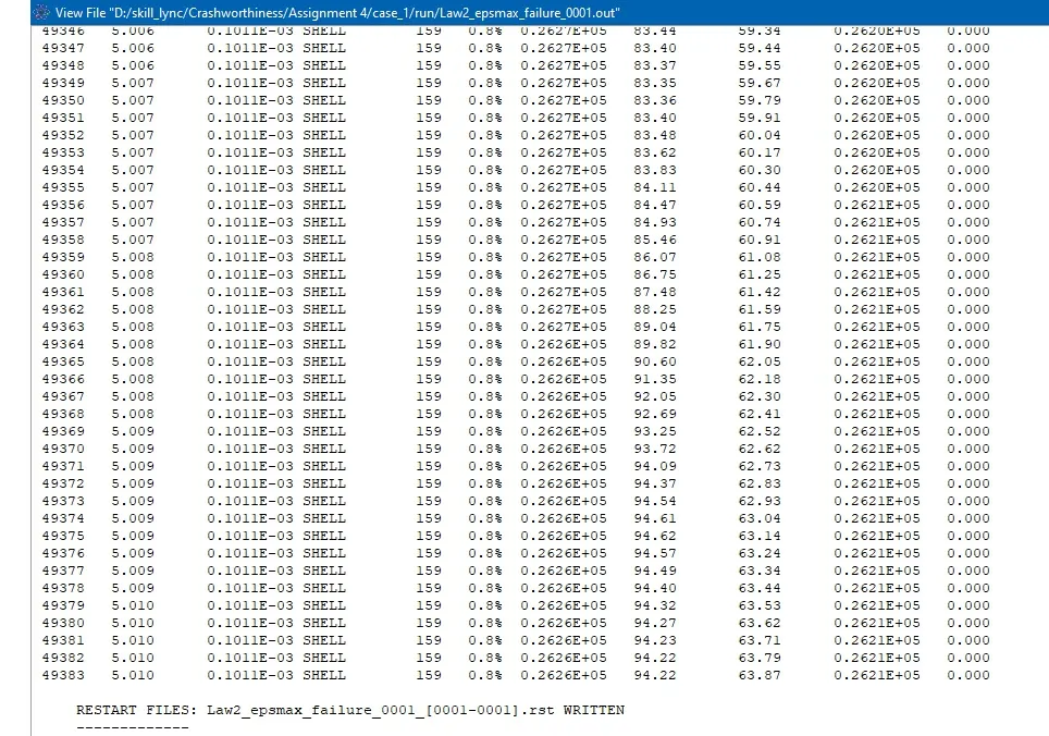
From the above image the total number of cycle at the end of 116.88s is 49384 and energy error is 0.8% which indicates that the simulation is stable and there is no energy created in the simulation and mass error is 0.0.

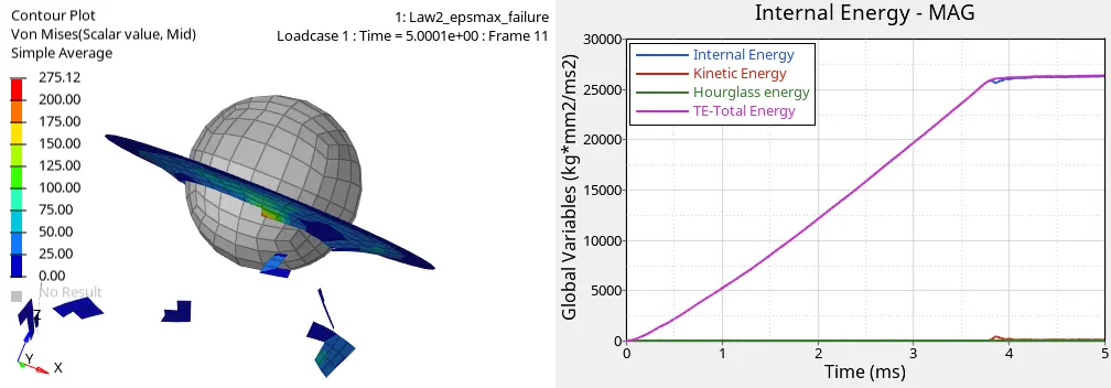
The above graph shows the internal, kinetic, hourglass and total energy in the simulation. from the graph it can be seen that their is no hourglass energy produced in the simultion, the internal energy increases as time increases this is because of elements absorbing the forces acting on them.

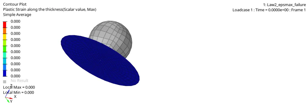
plastic strain contour graph

in the above image we can see that the elements are deleted when they reach 15% plastic strain after the yield stress value.

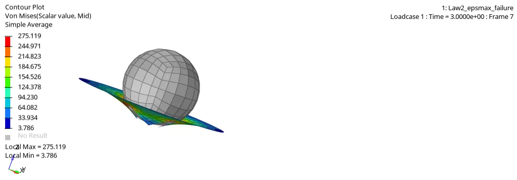
it can be seen that the elements are being deleted when they reach the 15.1% plastic strain after the yield stress of 290Mpa, the maximum stress in the simulation is 275.11 MPa.

elements break because the Johnson-Cook failure criteria model is applied to the simulation model which considers both tensile and compressive failure into account, when the elements plastic strain reaches Eps_p_max value they are deleted from the simulation, which is seen in the model above.

Case 2:

Change the failure card as shown below.

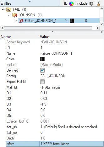
edited failure card

here Ifail_sh is Shell failure flag and is set to 1 which will generate crack in the shell element when Ixfem is set to 1, Dadv is the criterion for the crack advancement.

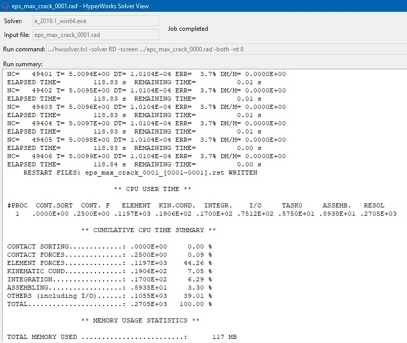
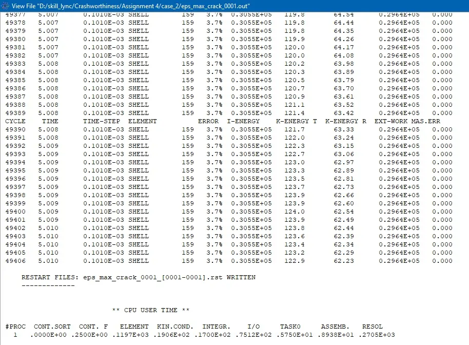
images above show the energy error, mass error, number of cycles and the time.

energy error is 3.7% which is acceptable result. the simulation time taken is 119.56s which is higher than the previous simulation.

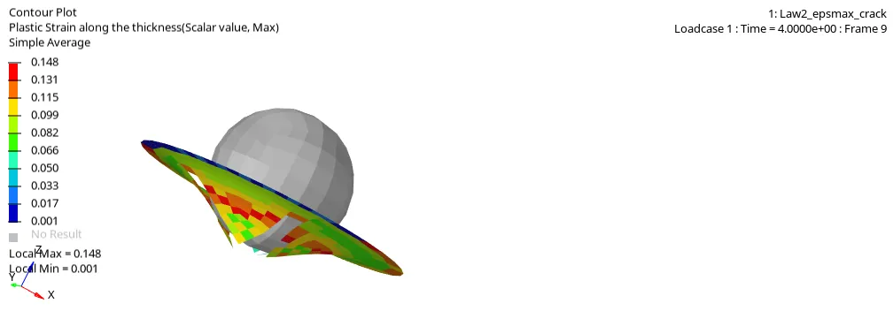
Plastic strain contour plot.

image above shows elements being cracked at the centre before getting deleted.

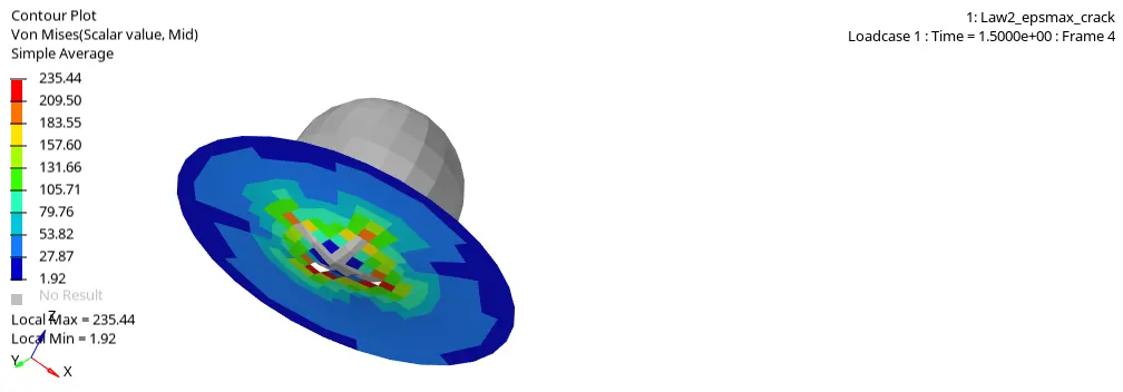
the maximum stress in the simulation is 310 MPa which is higher than the previous simulation. crack developement can be seen in the simulation.

since the crack advancement is set the maximum value of 1 and Ifail_sh is activated for shell elements, we can see the crack being generated in the simulation.

CASE 3:

Delete the failure card from the simulation and run the simulation

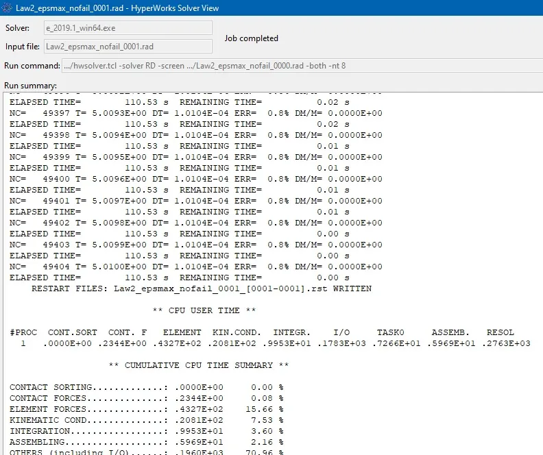
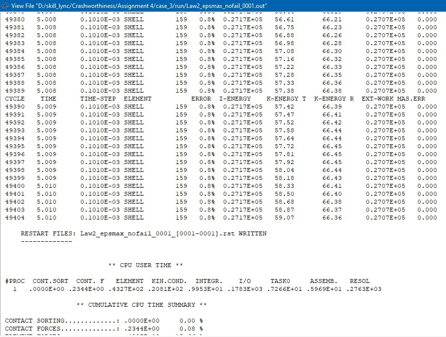
energy error is at 0.8% which is less than 15%, hence the result is acceptable. time elapsed for this case is 111.20s.

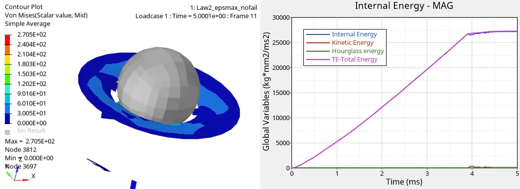
hourglass energy in the simulation is zero, this is due to QEPH24 element formulation, the internal energy in the model increses with time similar to both the previous simulations. The maximum stress in the model is 270.5MPa, and their is no crack observed in the simulation.

hourglass energy and kinetic energy in the system are near about zero.

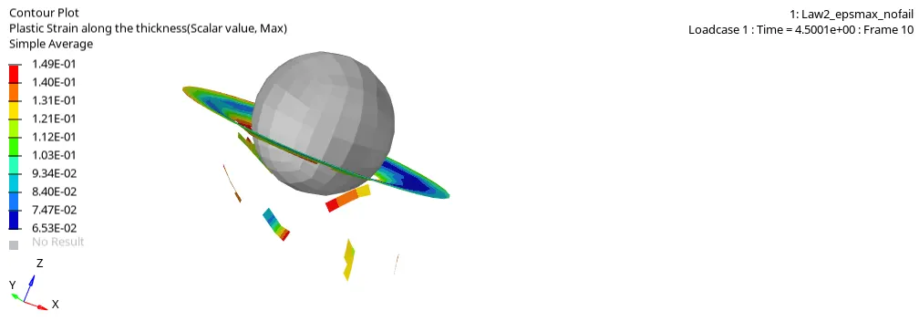
Plastic strain contour.

the elements are deleted in this simulation.

CASE 4:

Running the model with zero EPS_p_max value.

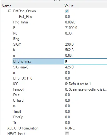
material card image.

time for the simulation is 111.79 sec.

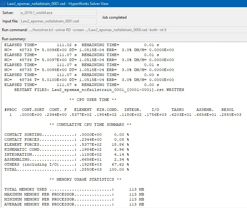
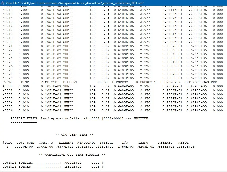
energy and mass errors are in acceptable range.

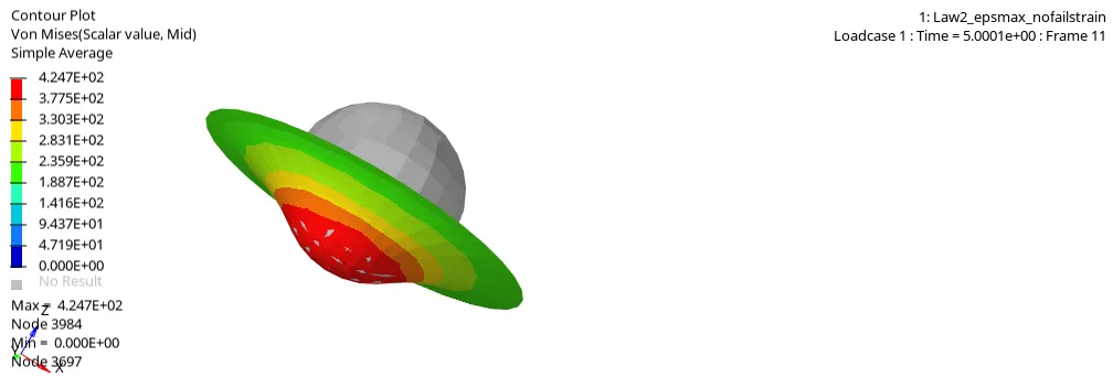
Maximum stress is 424.7 Mpa and there is no failure of element observed.

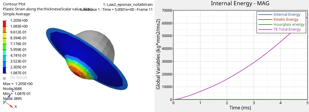
the above images shows that their is no hourglass energy generated in the simulation and internal energy and total energy of the simulation model intecepts eachother and increases with time.

In this simulation model the elements do not fail as the their is no failure criteria applied to the model, and Eps_p_max (Failure plastic strain) value is deleted which sets it to the default value of 103, and the maximum stress value is set to 425MPa due to which the maximum stresses in the model is seen to be 424.7MPa, and their are no elements deleted in the model.

CASE 5:

Changing the law 2 (elasto-plastic material) to law 1(linear elastic material)with same values of E (youngs modulus), density and poissons ratio.

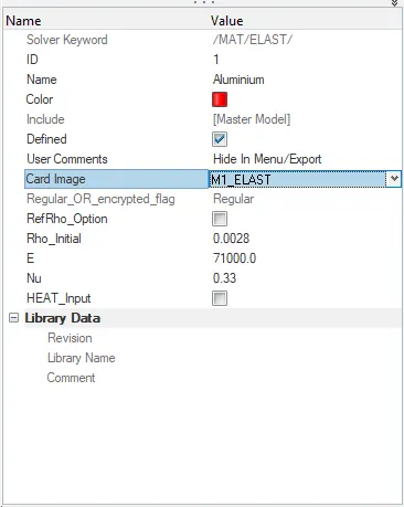
Material card for the simulation.

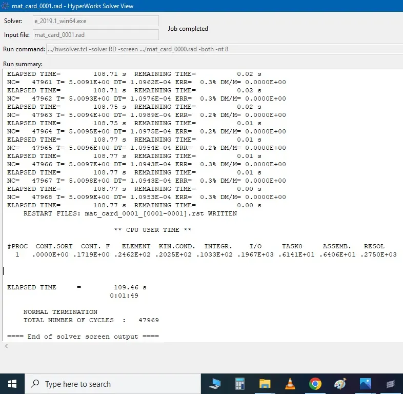
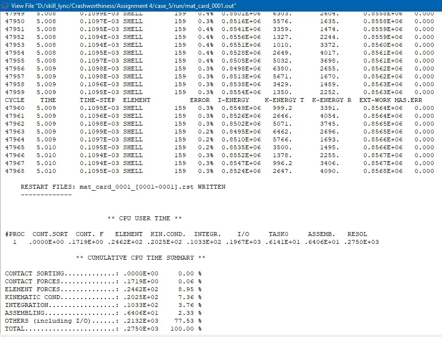
Run time is 109.46 s. energy error is 0.3%

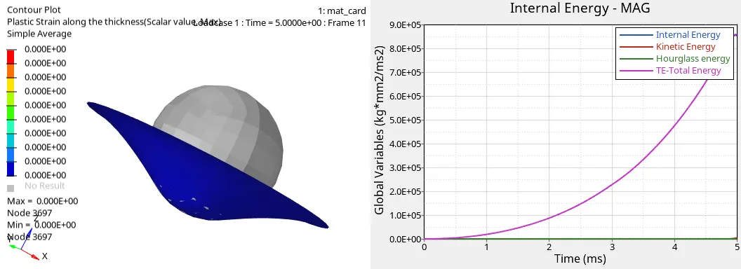
No hourglass energy generated in the simulation and internal energy and total energy of the simulation model intecepts eachother and increases exponentially with time.Since the material law applied is linear elastic, their is no plastic region in the material hence no elements fail and no plastic strain is recorded in the simulation.

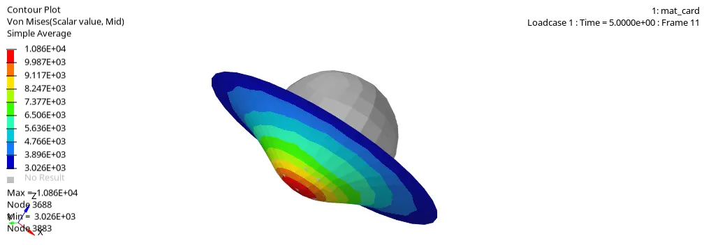
the material has no maximum stress defined and the stress strain relation is linear, hence their is no failure of the elements.

CASE 6:

Law 36 which is a isotropic elasto-plastic material using user-defined functions (curve).

create a curve with to apply in the material model N_funct.

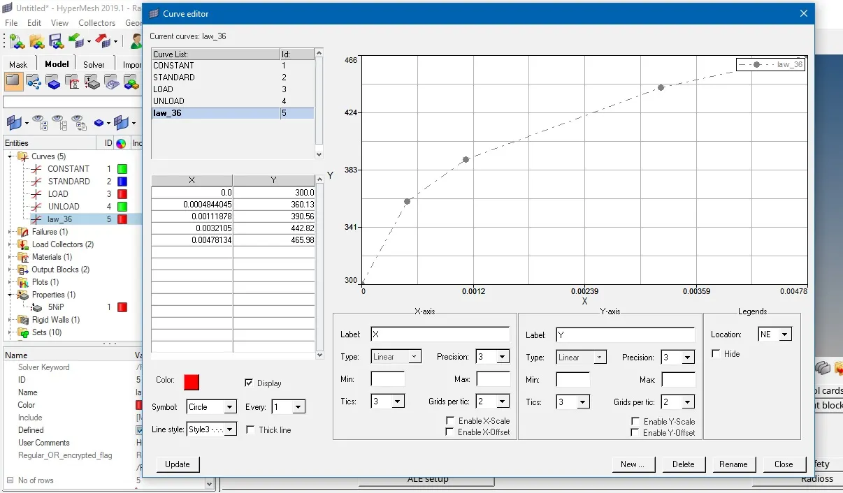
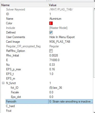
Material card selection and curve selection.

N_funct is Number of functions which can be between 1 and 100 depending on the requirments of the simulation.

Fscale default value is 1.

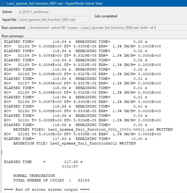
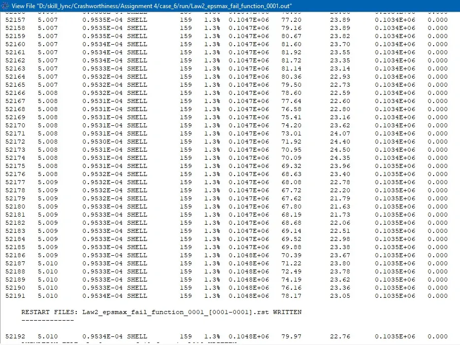
energy error and mass error are in acceptable range for the simulation, and time elapsed is 117.63 s.

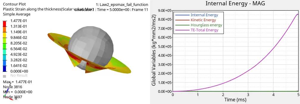
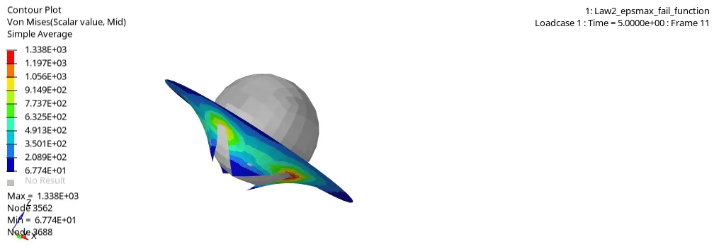
their is no hourglass energy generated in the simulation model, the internal energy increases with time as seen in the image.

CASE 7:

change the material card to Law 27 ( elasto-plastic Johnson-Cook material model with an orthotropic brittle failure model )

this law combines johnson cook material with the brittle failure method, this law is applicable only for shell elements.

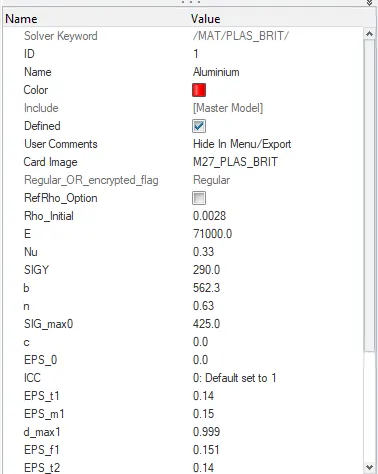
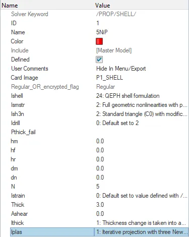
material card for LAW 27.

where,

EPS_t1 is tensile failure strain at which stress starts to reduce in the principal strain direction 1.

EPS_m1 is maximum tensile failure strain in principal strain direction 1 at which the stress in the element is set to a value dependent on dmax1

EPS-f1 is maximum tensile strain for element deletion in principal strain direction 1

dmax1 is maximum damage factor in principal strain direction 1 which is at default value of 0.999.

EPS_t2, EPS_m2 and EPS_f2 are for direction 2.

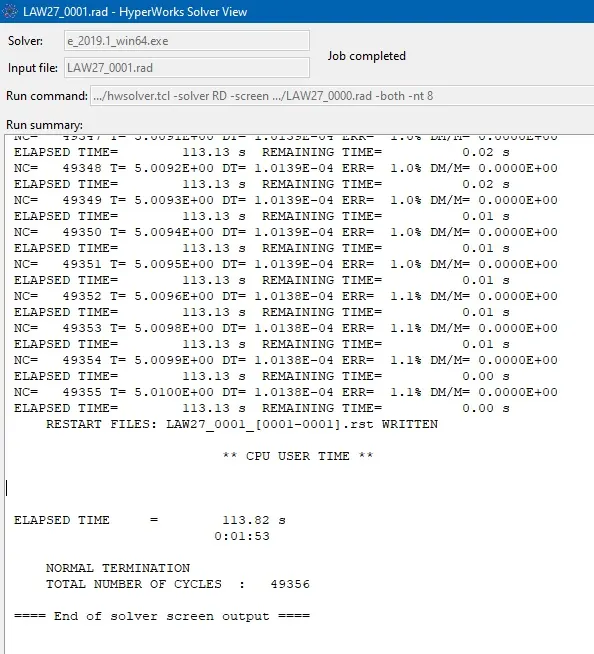
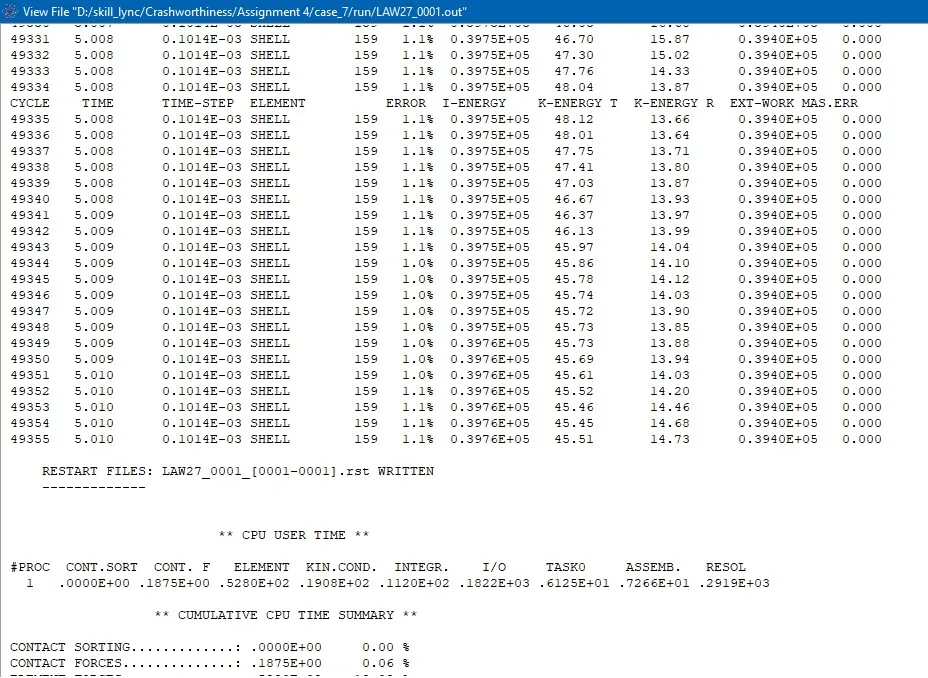
energy error and mass error values are in acceptable range for the simulation, time for elapsed for the simulation is 113.82 sec.

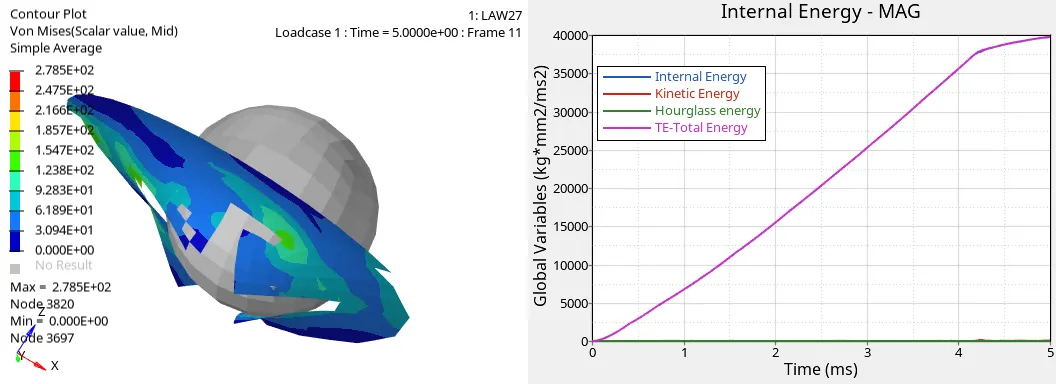
their is no hourglass energy in the simulation model, the internal energy and total energy increase with time and then tends to flaten after 4ms as seen in the image above.

Elements are deleted in the simulation due to EPS_t, EPS_m and EPS_f values.

the maximum stress developed in the simulatioon is at 278.5 MPa, which is below the Plasticity yield stress value of 290 MPa.

the material breakes after the cracks reach the end of material boundary as seen in the simulation image.

Once the EPS_p (plastic strain) reaches EPS_p_max , in one integration point, the element is deleted.

Conclusion:

• By observing the Von Mises and Ultimate stresses generated in the materail during simulation and comparing with the actual data (experimental) of the aluminium material, it can be concluded that the Case 2 ( Law 2 - Johnson Cook model) represents the on field testing condition of the material.

• The material failure (element deletion) occurs only after the crack propagation.

• Comparison between different material cards and failure cards has been carried out by applying them to the given simulation model. Element behaviour and stress development has been discussed. Based on the observation of results: case 2 presents the best on-field scenario in the simulation.