Assignment 4-RADIOSS Material Laws Challenge

AIM:

To import the given model and run the analysis with different material laws and other modifications and observe the results.

OBJECTIVE:

To perform the simulations of the given starter files and compare the results with other outputs. There are 7 cases with given parameters and they are to be compared with output animations and plots. The files to be worked on are the FAILURE_JOHNSON_0000.rad file and the LAW27_0000.rad file.The 3 slides are given with parameters

• The failure johnson rad file is imported and run with base simulation.
• The failure johnson rad file is imported and run with changes of Ifail_sh = 1, Dadv = 1, and Ixfem = 1.
• The same file is run with fail/JOHNSON card deleted.
• The previous rad file is imported and run with EPS_p_max value deleted
• The previous rad file is imported and run with change in values for density, E, nu ,young's modulus
• LAW27 rad file is imported and run with givenshell properties
• LAW27 rad file is imported and run with given shell properties and new curve is created.

PROCEDURE:

Case 1:

Open Hyper mesh, go to >> import >> solver deck option >> browse File > FAILURE_JOHNSON_0000.rad file is selected and imported .

In Base simulation, the simulation is run with the default values without any changes.

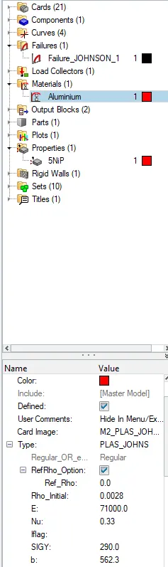
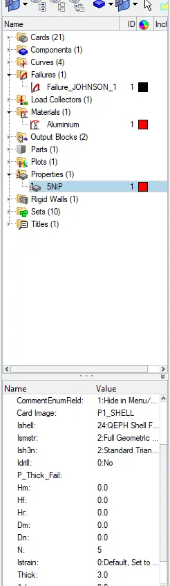
Next, Go to Analysis >> Radioss select save as and the file is saved in local directory . After saving, check the 'include connectors' box and type in '-nt 4' in the options text box and click 'Radioss'. Here nt refers to the number of threads assigned to the simulation from the cpu.

After radioss is clicked , a window opens showing the process of radioss solver and then various animations file and files to plot the energies are created in the local directory.

After radioss is run and files are created it is visualized using hyperview.

After accessing Hyperview, we should input the simulation file. For this, use h3d file that was generated when RADIOSS processed the starter file. It is generated in the files swhich are shown in the picture above. After selecting it, we can click 'apply'

After accessing Hyperview, we are asked to input the simulation file. For this, we shall be using the h3d file that was generated when RADIOSS processed the starter file . It should be generated in the same folder. After selecting it, we can click 'apply'. Doing so generates the simulation animation

We can change what is being represented by selecting the 'contour' option in the toolbar. In this case, we can change the result type to 'Von Mises' and change the averaging method to simple. Doing so creates the Von Mises stress

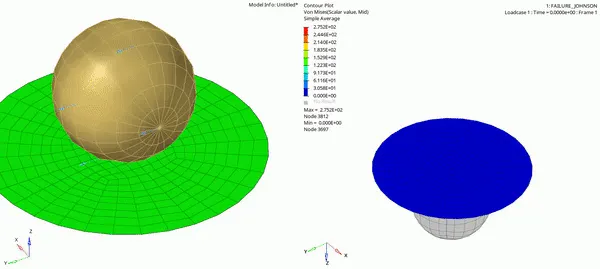
Next step is to carry out energy error and mass error checks and this is done by analyzing the RADIOSS engine output file. This can be accessed from the same directory as the starter and engine files and is denoted by the '.out' extension. We need to check the file that contains '_0001.out' by using any text editor.

On opening the file and scrolling down to the end, we can see the final energy and mass error values.

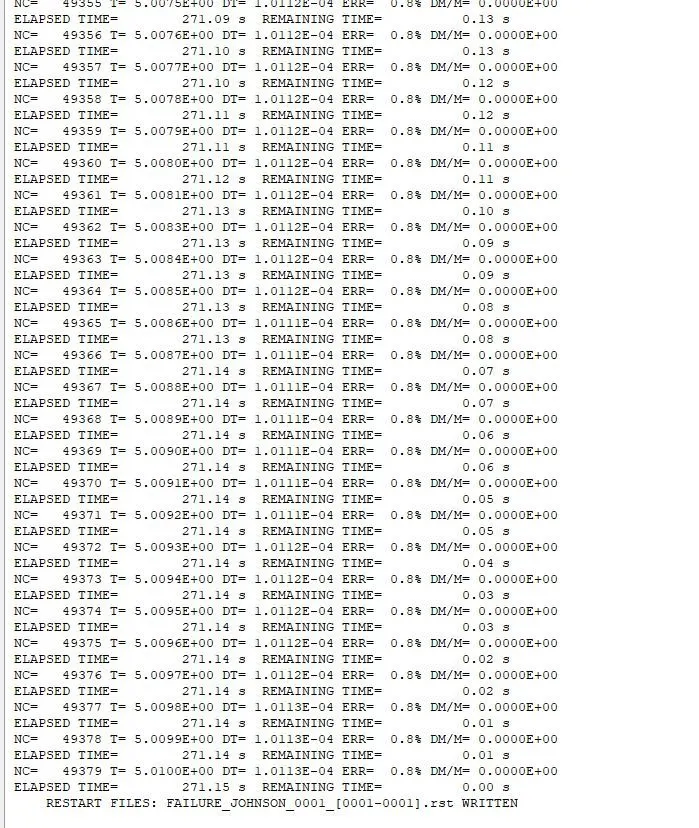
The final energy error is 0.8% and is acceptable range and mass error is zero.

TOTAL NUMBER OF CYCLES : 49380

In the Hypergraph section, we need to input a file to plot the graph. This file is available in the same directory as the starter, engine, and animation files. The file name ends with 'T01'.

CASE 2

The process is repeated with slight modification. Import “FAILURE_JOHNSON_0000.rad” via the solver deck.

This time, changes to the fail/JOHNSON card is made It can be accessed via the model tab, under the “Failures” submenu.

The following values are assigned as shown below (Ifail_sh = 1, Dadv = 1, Ixfem = 1)

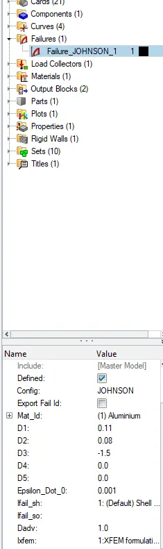
Now run the analysis and the file is saved as in a separate directory. With connectors checked and '-nt 4' typed in the options box, we can click the Radioss button to run the analysis.

After the solver window completes the analysis, as usual, switch to HyperView window and run the h3d file of the current analysis and set the Von Mises stress contours

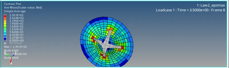
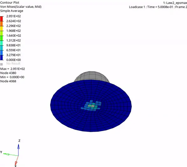
Now, check the energy and mass error on the RADIOSS output file in the .out file

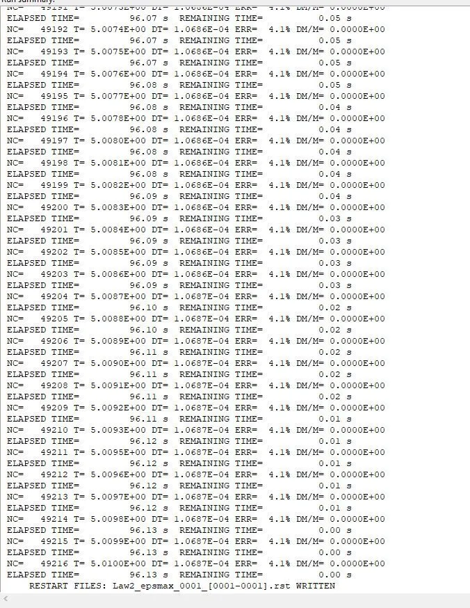
The energy error is lesser than 5% and mass error is zero

TOTAL NUMBER OF CYCLES : 49217

CASE 3

Open Hyper works and import the starter file created in the previous case.

In this case delete the fail/JOHNSON card. Go to Failures > Failure_JOHNSON_1.

Now run the analysis and the file is saved in a separate directory with connectors checked and '-nt 4' typed in the options box, we can click the Radioss button to run the analysis.

After the solver window completes the analysis, as usual, switch to HyperView window and run the h3d file of the current analysis and set the Von Mises stress , check the energy and mass error on the RADIOSS output file from the .out file

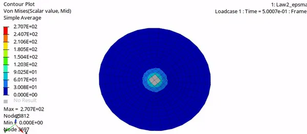
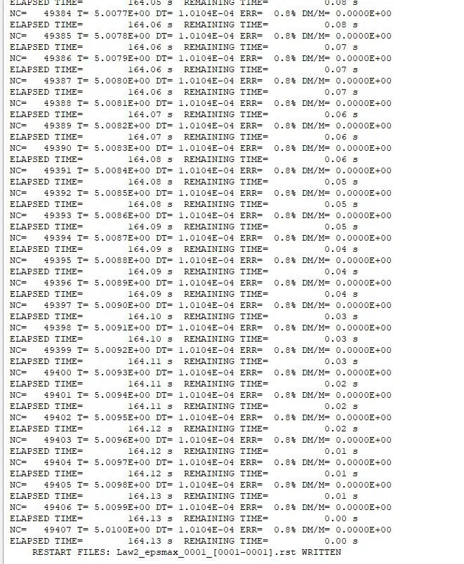
The energy error is 0.8 and the mass error is non-existent. Now we can switch to Hypergraph to plot the graphs.

TOTAL NUMBER OF CYCLES : 49408

CASE 4

In this case, import the case 3 starter file in radioss

here, delete the EPS_p_max value (make it as 0). Going to the model tab, we can go to Materials > Aluminium

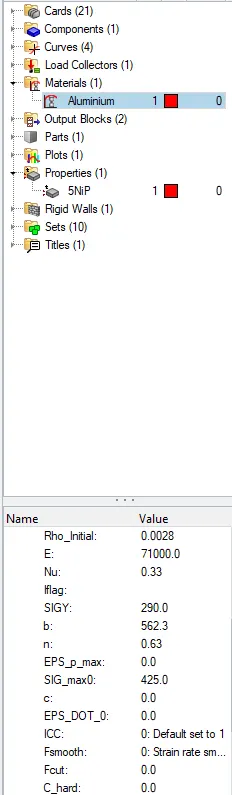
After that, we can switch to the Radioss analysis section via Analysis > Radioss, save the file as separate directory, check connectors and type in '-nt 4' in the options section and run the analysis by clicking 'Radioss'.

After the solver finishes its analysis, we can switch to Hyperview, run h3d file, activate the Von Mises contours and view the simulation

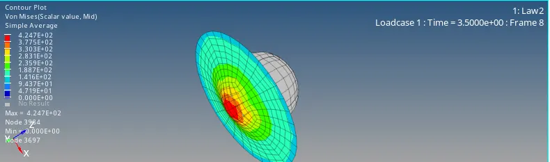
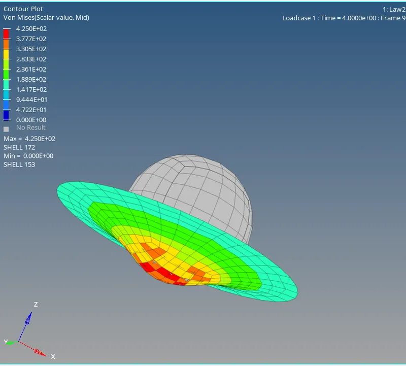
Now, check the energy and mass errors on “Law2_0001.out”

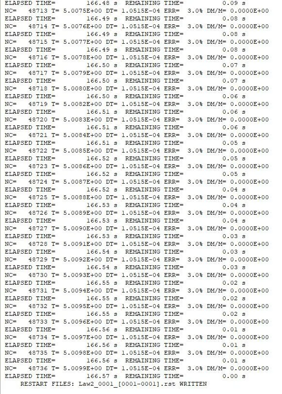
The energy error is less than 5% which is acceptable and mass error is zero

TOTAL NUMBER OF CYCLES : 48737

CASE 5

In this case import the main starter file FAILURE_JOHNSON_0000.rad.

go to Materials card > Aluminium and change the card image to M1_ELAST, which is Law 1.

Set the values for Rho_Initial, E & Nu as Rho_initial = 0.0028, E = 71000.00, nu = 0.33.

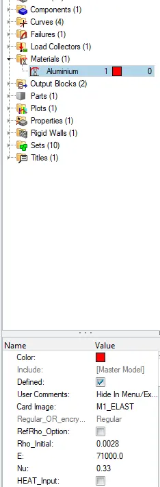
Now run the analysis and save the file and enable connectors and type '-nt 4' in the options box. Then, click on radioss and let the solver run the analysis.

After the solver completes the analysis, we can switch to Hyperview, import the h3d file, enable the Von Mises contours and view the simulation

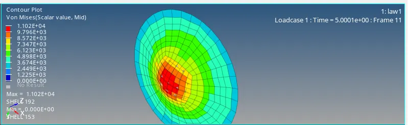
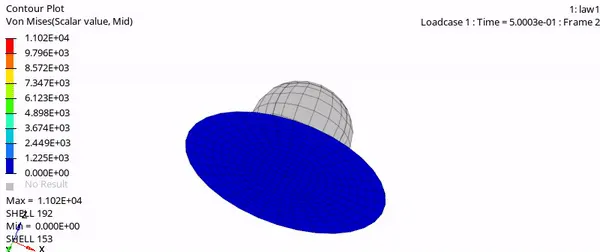
Now, check the energy and mass error on the RADIOSS output file saved as .out

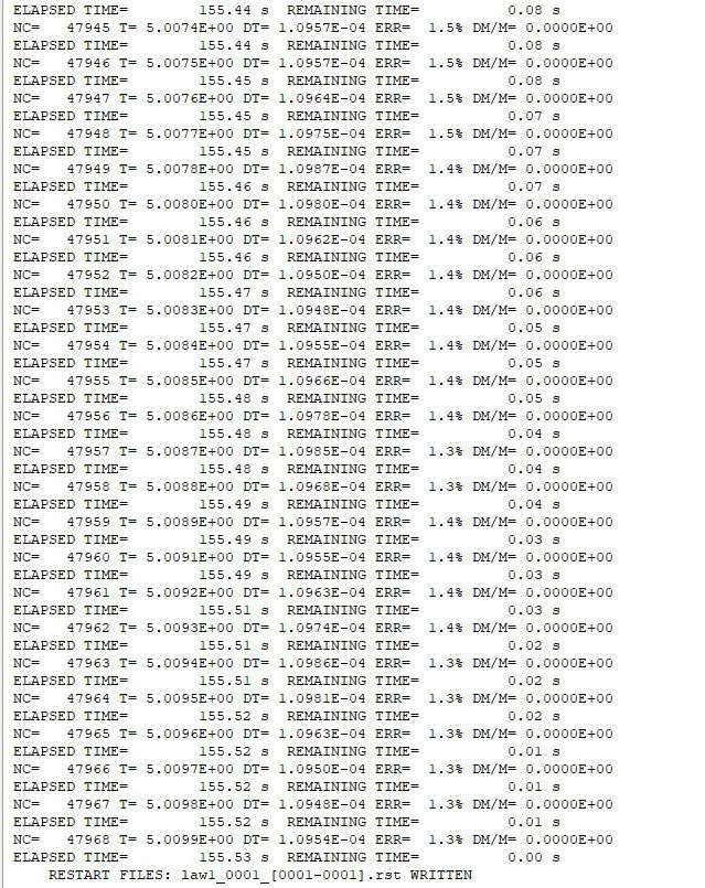
The energy error is less than 5% and is acceptable the mass error is zero. switch to Hypergraph to plot the graphs for this simulation

TOTAL NUMBER OF CYCLES : 47969

CASE 6

In this case, import the 'LAW27_0000.rad' file.

Use the given shell properties in this case. Go to Properties > 5NiP. In the utility window set the following attributes as follows as I_shell=24, I_smstr=2, I_sh3n=2, N=5, I_thick=1, I_plas=1

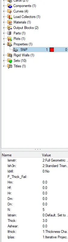
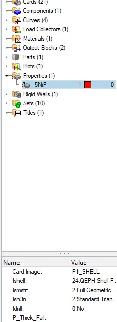
Now, run the analysis via the Radioss tool. This time, we can save the file as 'Law27_0000.rad' and enable connectors and type '-nt 4' in the options box. Then click on radioss and let the solver run the analysis.

After it's done, we can generate the simulation via Hyperview with the Von Mises contours enabled as shown

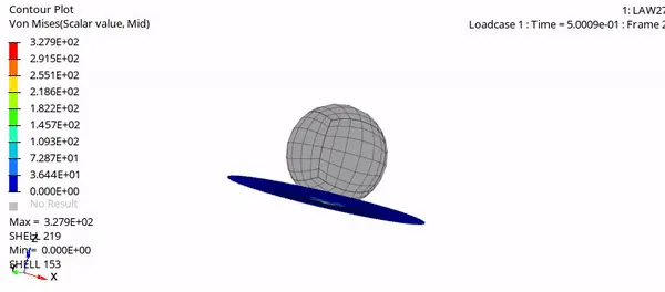
we can check the energy and mass errors on “Law27_0001.out”

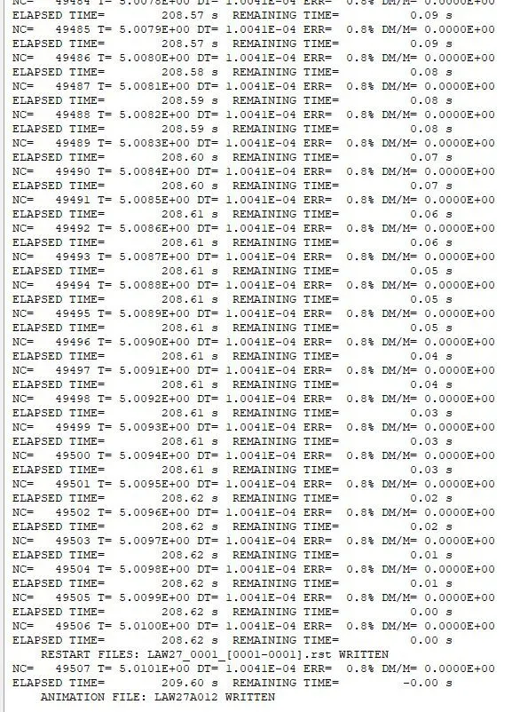
The energy error is almost 0 and the mass error is zero.

TOTAL NUMBER OF CYCLES : 49508

CASE 7

In this case import 'LAW27_0000.rad' .

Go to the model tab and create a new curve . Right-Click >> Create >> Curve

A new curve is created and name it as case 7

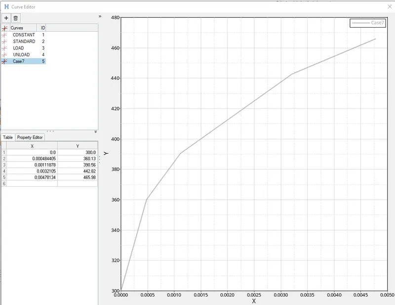
In Materials >> Aluminium change the card to M36_PLAS_TAB (Law 36). After that, set the values for Rho_Initial, E & Nu as
Rho_initial = 0.0027, E = 71000.00, nu = 0.33.

Add the curve using the N_funct attribute. We can change its value to 1 and select the reference curve that is created

Now run the analysis using the Radioss tool via Analysis > Radioss , name the file “LAW36_0000.rad” and save it in local directory

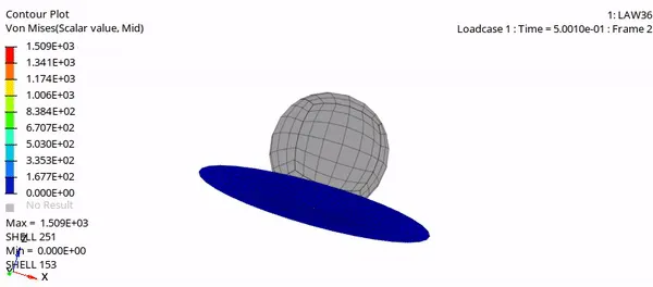
After the analysis is complete, we can switch to Hyperview and import h3d file. With Von Mises contours enabled, we can view the simulation

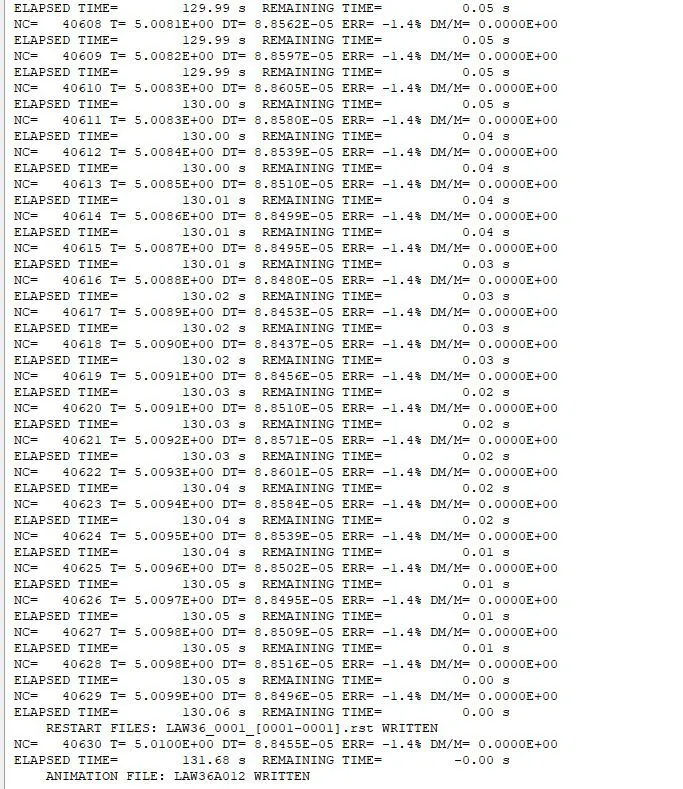
An energy error of -1.4% is very acceptable since it's very close to 0. As usual, the mass error is zerot.

TOTAL NUMBER OF CYCLES : 40631

OBSERVATION:

Case 1:

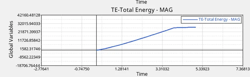
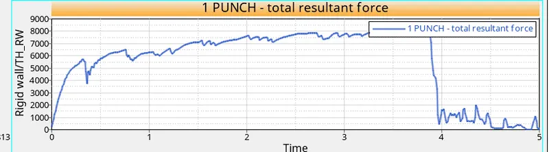
In case 1, it has the Fail/JOHNSON card as well as EPS_p_max value assigned, with Ixfem value as 0. Here the elements are deleted as soon as they cross the EPS_p_max value.Internal energy and rigid wall forces, are reactions to the force generated by the sphere on the sheet. Energy increases gradually until many elements are deleted at around the impact This causes vibrations and that results in increase of kinetic energy at the same point.

The rigid wall forces keeps increasing and decreasing when the elements are deleted, and when elements are deleted on impact the graph drops, since there aren't many elements opposing the impact of the sphere.

Case 2:

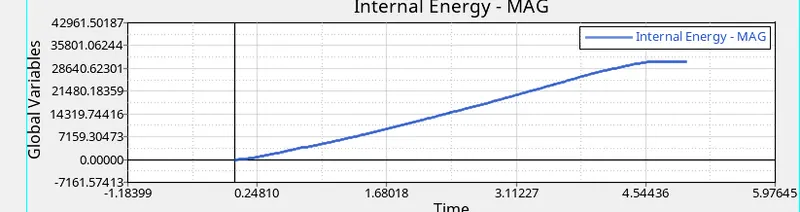
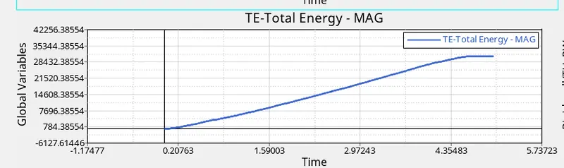
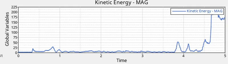
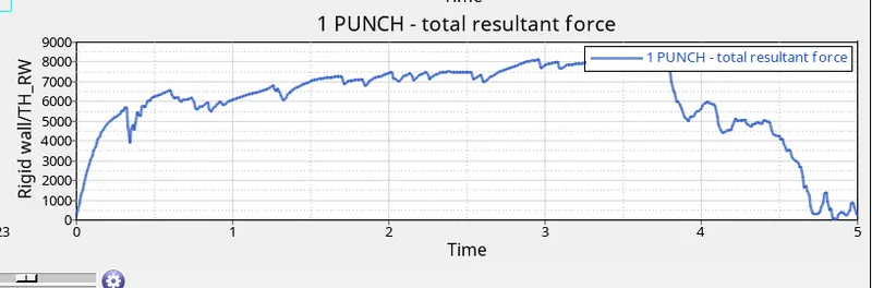
with case 2 the Ifail_sh, Dadv, and Ixfem values are changed in the Fail/JOHNSON card. Ixfem decides the way the elements react. With its value equal to 1 here, it means the elements will crack and then fail andwith Dadv, crack propagation can also be seen here, with elements being deleted only when the crack reaches them. This is the most suitable case for this simulation.

Here the rigid wall is in motion because there is external force applying on the object. So that is why the rigid wall forces start increasing from zero and when it collided with the plate, the energy got transferred to the elements, that's the reason the rigid wall forces get decreased again to zero.

Case 3:

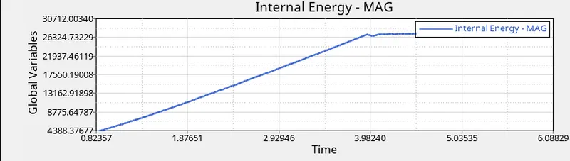
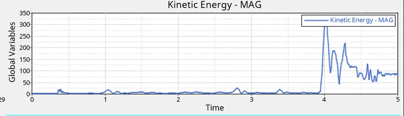
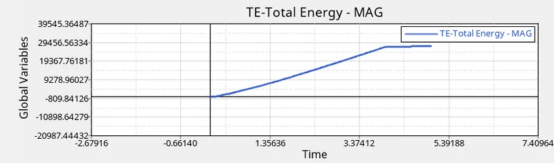
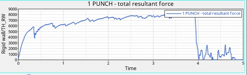
Fail/JOHNSON card is deleted in this case, the EPS_p_max value is to be factored for element deletion. The elements fail gradually here when compared to the elements in case 2 .

There is a linear increase in internal and total energy until elements are deleted from the model. The energy absorbed by the elements decreases due to their deletion.

This also explains the sudden drop in rigid wall forces at the same timestamp due to most elements that were in contact with the sphere during collision being deleted. The rigid wall force is basically a measure of the opposing force generated by the metal sheet against the sphere. Fluctuations occur in graph when elements are deleted. When there are no elements to oppose the incoming sphere, there won't be any rigid wall forces.

Case 4:

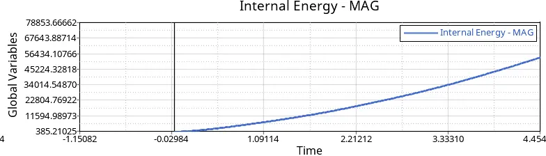
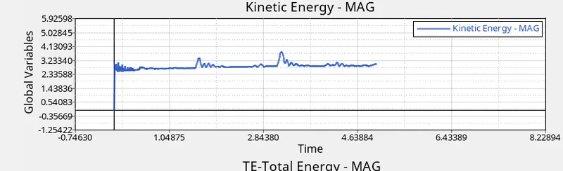
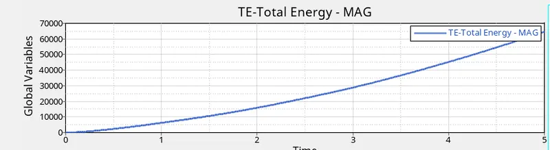
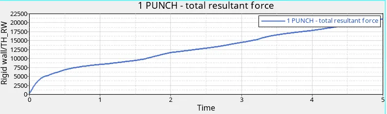
In case 4, the metal sheet is able to withstand stress on impact and element is not deleted since the value for EPS_p_max was deleted and RADIOSS assigns it the default value . The elements cannot be deleted since the failure card is deleted and is not cracked so the material is bending to the maximum .

The total energy is gradually increasing over time.

The kinetic energy increases suddently at the start of the impact and ove time it fluctuates and the spikes are when maximum load is applied on elements due to elasticity

Case 5:

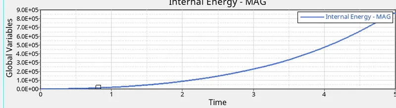
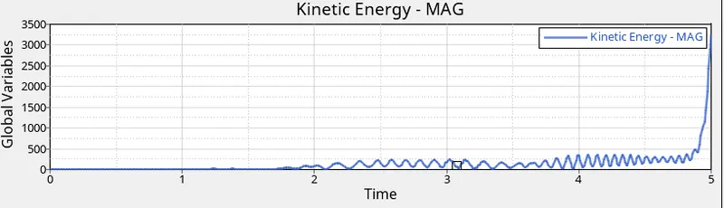
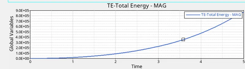
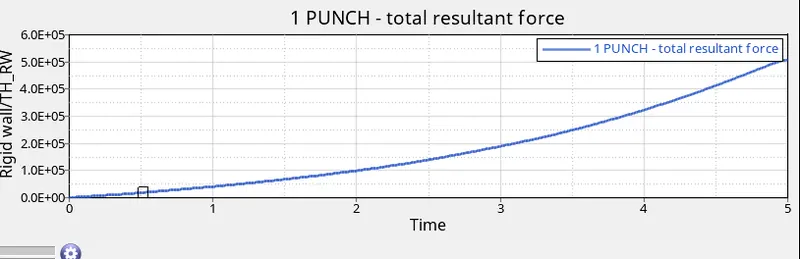
In Case 5, the metal sheet is LAW-1 material which represents properties of elastic material.This case makes use of the M1_Elast card and as we can see, the metal sheet absorbs the full impact of the sphere. This material law is used to model only elastic materials.

This is the reason for no element deletions and cracking. Due to the elasticity it also can absorb an extremely large amount of energy, which explains the peak at the end of the kinetic energy plot . Bending due to a lot of energy also results in very high stresses .

The kinetic energy gradually increases as the metal sheet is bending to the maximum while the sphere is impacting on the metal sheet.

Due to the elastic property the internal energy and rigid wall forces keep increasing . The internal energy of the metal sheet increases due to the of the kinetic energy from the impact of sphere and decreases once the sheet returns to the original shape.

Case 6:

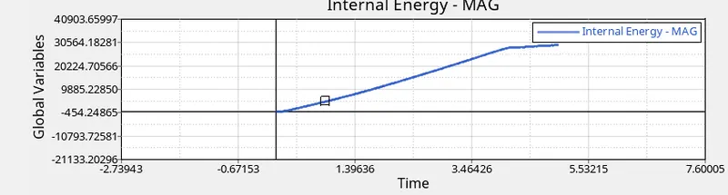
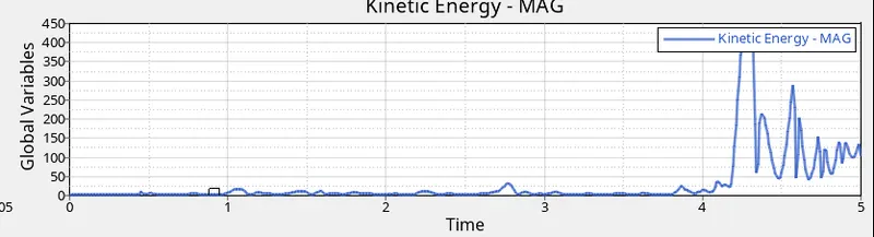
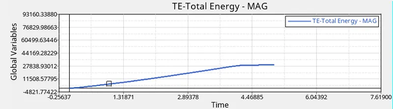
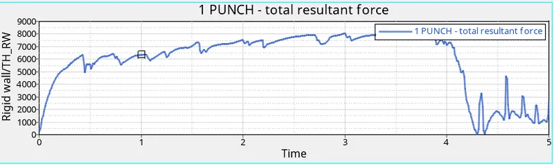
In case 6, the use of the M27_PLAS_BRIT material card that is used for Johnson-Cook material model with comparison to case 7 ,absorbs more force and undergoes more deformation of material before the elements are deleted at around 4m/s .

Due to the loss of energy through element deltion, the graph plateaus at around the 4 /s mark.

After the elements deleted there is no elements to stop the impact of sphere, the rigid wall force graph decreases at around 4ms. The ups and downs represents the time when elements are getting deleted.

CASE 7:

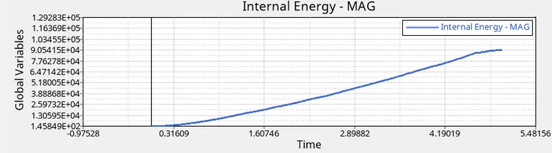
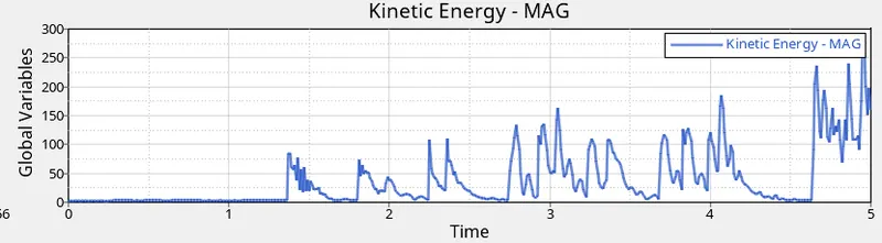
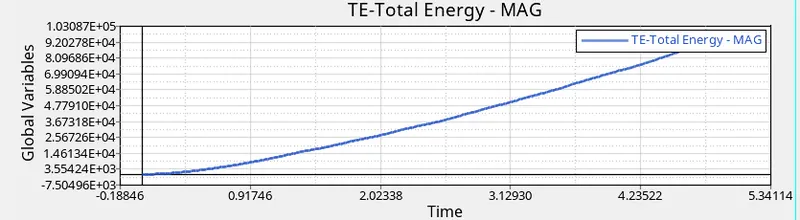
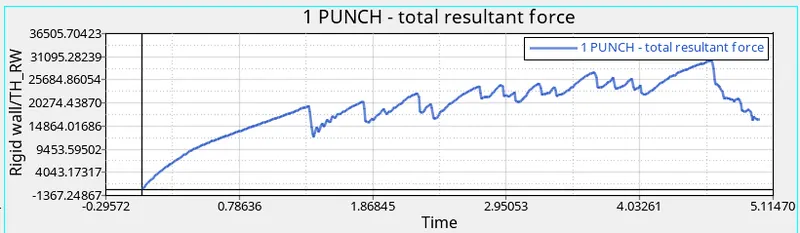
In case 7 it is observed from the simulation that this material does not bend on impact due to the applied force and immediately breaks. It does not crack and in place of the deleted elements the sphere is seen. the stress concentration is only around the region of impact and these stresses are not impactful in the whole metal sheet

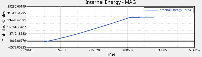
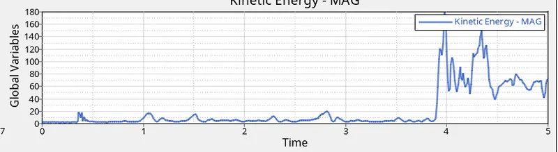
The curve is gradually increasing with internal energy and time till past the 4m/s mark and many elements get deleted on impact. When the elements are deleted on impact the energy on each element gets decreases, which results in the decrease of the curve.

The spikes represent the deletion of element on impact. The resultant force gradually increases past the same 4m/s mark which is when the metal breaks with the impact of sphere. after that, the rigid wall forces is decreased and that results in that drop of curve at the 4m/s mark. The first drop in graph occurs when the sheet breaks the first time on impact.

TABLE FOR COMPARISON OF CASE RESULTS

CASE	SIMULATION NAME	No.of cycles	mass error	energy error (%)	simulation time (s)	elements under stress
1	Law 2 (Johnson-Cook model)	49380	0	0.8	190.33	deleted
2	Law 2 (Johnson-Cook model)	49217	0	4.1	96.79	elements are cracked and then deleted
3	Law 2 (Johnson-Cook model)	49408	0	0.8	164.78	deleted
4	Law 2 (Johnson-Cook model)	48737	0	3	167.28	Cannot be deleted
5	Law 1	47969	0	1.3	156.19	cannot be deleted due to elastic property
6	Law 27	49508	0	0.8	209.63	deleted
7	Law 36	40631	0	-1.4	131.72	deleted

Conclusion:

Comparison between different material cards and failure cards has been carried out by applying them to the given simulation model. Element behaviour in stress increase is observed. Based on the observation case 2 presents the best on-field scenario in the simulation.