Study model behaviour and Controlling animation using engine file in Radioss.

Aim: Study the behaviour of provided model with and without changing the material properties of it and also see how can we control animation using engine 0001.rad file for the same model.

Procedure:

Now, to study all these behaviour of model in radioss we need a starter file i.e. 0000.rad and engine file i.e. 0001.rad for the same model.

Now, the question arises what is this stater and engine file. Starter file is an ASCII file that contains the model definition, it means information of set of nodes or elements in the model, material information, properties of model and its interfaces. And engine file is an ASCII file that describes the run control of animation file for the model i.e. target timesteps.

ASCII - American Standards Code for Information Interchange.

Now all this information was already provided to us. Now our job is to import these files in radioss to study the model behaviour.

To import file, we follow below mentioned step. As mentioned, starter file if the file which contains all information for model so we will import only starter file and engine file will be used to control the animation.

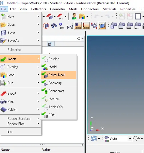
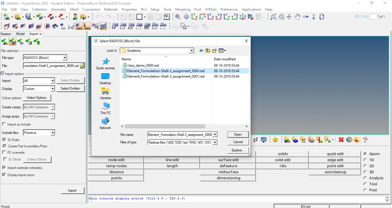
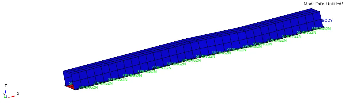
So, this way import will be done and we will see our model in graphic area. Than we can start analysis on this model, as it checked properly and then will be sent for analysis. So, to start analysis we need to switch to Analysis panel and choose radioss option there.

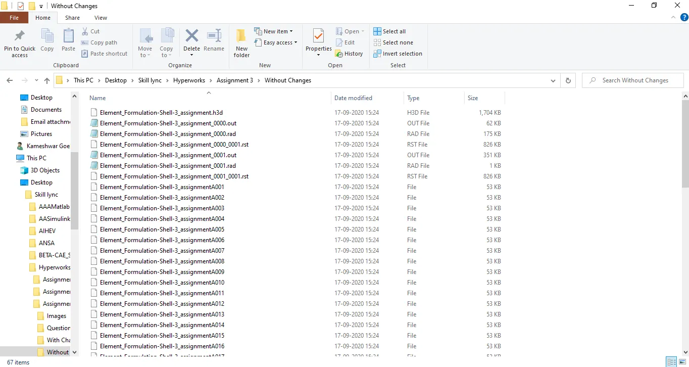
So, under radioss we need to take care of several parameters asked like input file designation as several file will be constructed so it is always better to save them in a designated new folder so that confusion won't come and also to meet computer specification it is better to give command -nt 4 in options so solver can run smoothly. Then click radioss to start analysis. During running you will observe this kind of window and at end of it you will find multiple files in your designated folder like this:

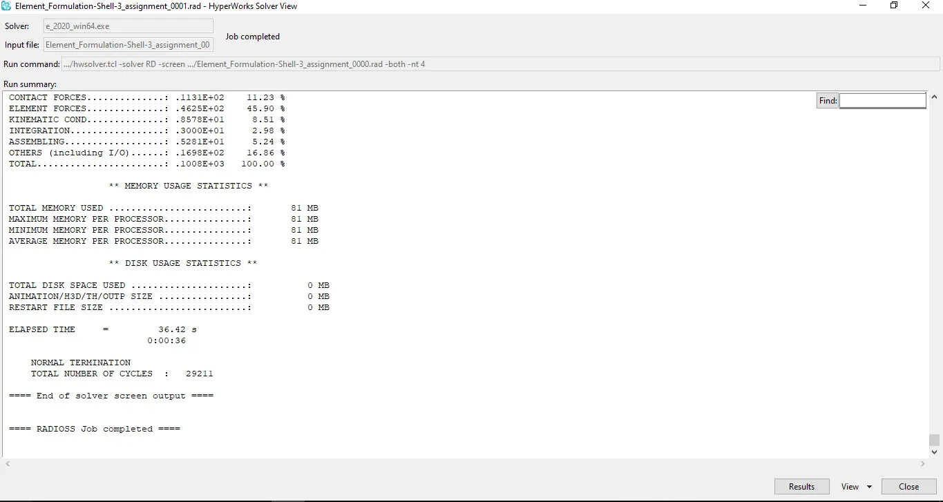
Now, as all the analysis is done and to see kinds of results, we need to switch the view type to different type like from HyperMesh to HyperView or HyperGraph 2D. But before that we need to understand few things from the data, we got in the designated folder during solving of model.

If we see that folder, we will find several files of different extensions like .h3d, T01, 001.out etc. So, in radioss h3d file is the file for animation which is actually a combined file of all A001-A059 file formed in folder and the number of A file in folder depends on the frequency we set in engine file. T01 file is the file used for plotting different kinds of plots, And 0001.out file will contains several information out of which we have parameters of concerns like energy error and mass error checks.

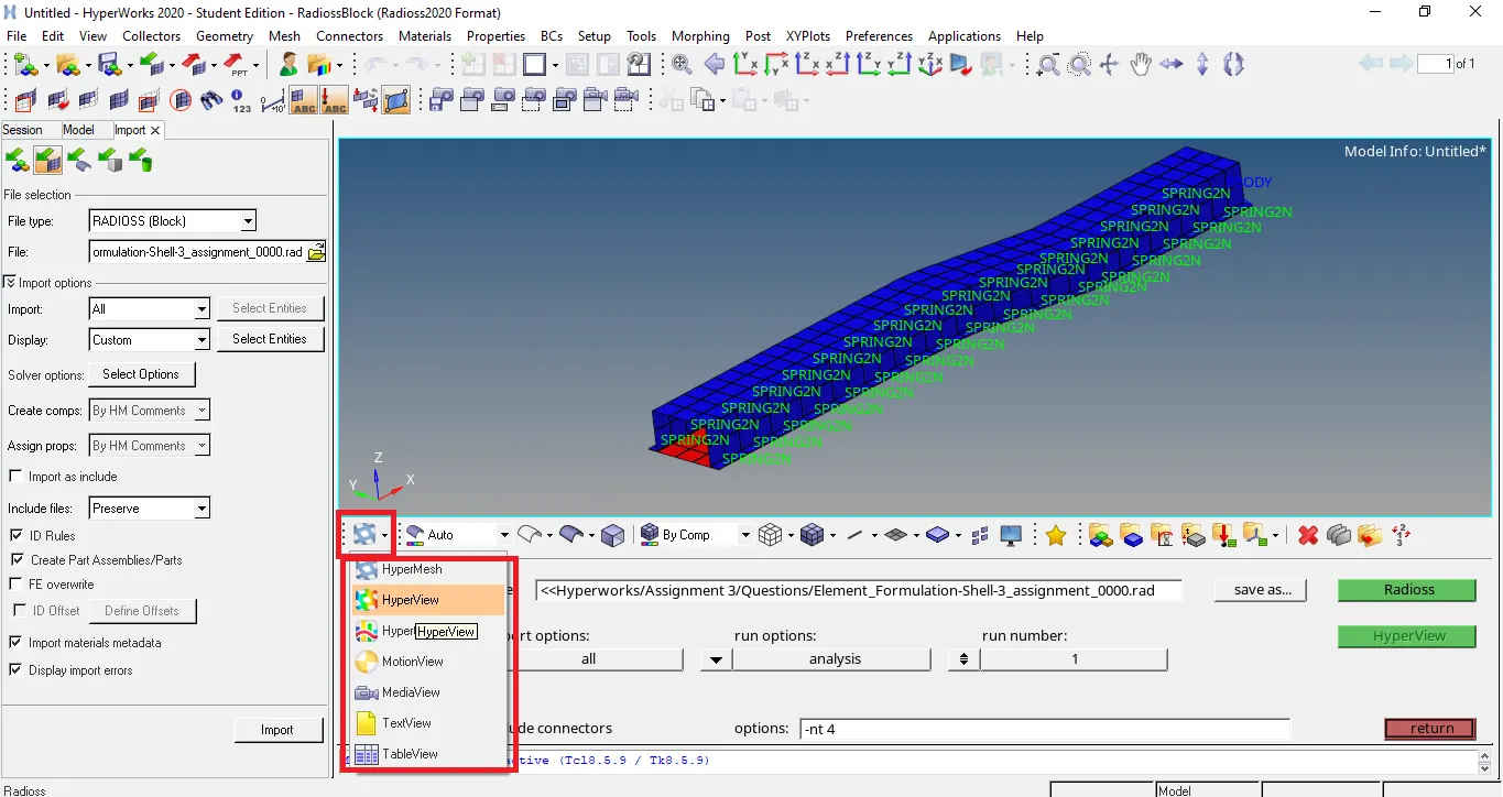
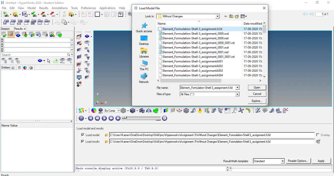
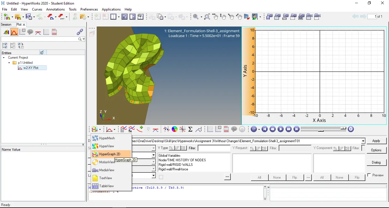
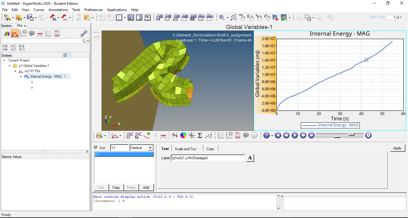
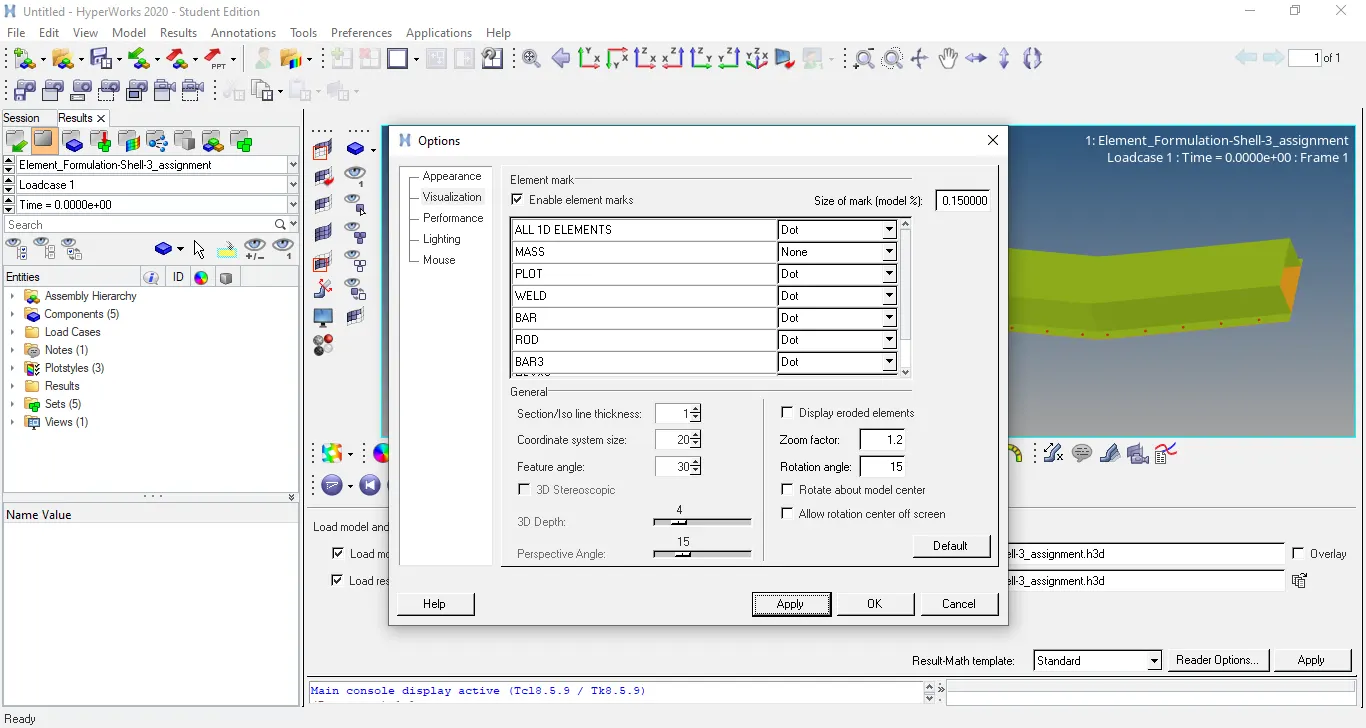
This way we can open h03 and t01 files in designated view type. Also, to enhance model specification in graphic area we can use option under Preference - Options. Like for this model we need to see spot weld points (1D elements). So, using this option we increased size of view to view where are they located.

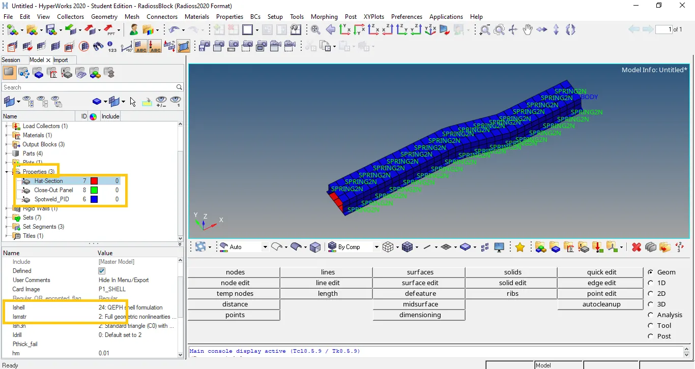
So, based upon all these steps we found several results with changing properties of the model. Now to change model properties as per given values we followed this process:

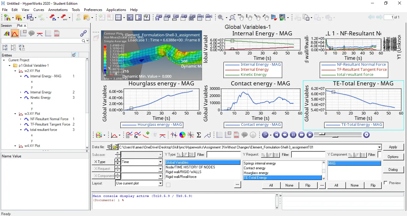
Now, without making any changes to the properties we got these results.

But before storing all these results there is a condition, we need to check always i.e. we need to check values of energy error and mass error from 0001.out file created in designated folder whether they are acceptable or not.

So, for the simulation type without property change we observed that energy error is fluctuating from 0.0% - (-10.3%) and mass error was 0.1659E-03 for every time step which depends on frequency, we set in engine file. Now, to understand this % we should first know the facts behind energy error what does it mean:

The Energy Error computed by Radioss is a percentage.

• If the error is negative, it means that some energy has been dissipated.

  In case of under integrated elements, the Hourglass energy can also explain a negative Energy Error since it is not counted in the energy balance. The normal amount of Hourglass energy is about -10% to -15%.

• If the error is positive, there is an energy creation.

  In case of using QEPH shell formulation (I_shell=24) or fully integrated elements, the Energy Error can be slightly positive since there is no Hourglass energy and the computation is much more accurate. An error of +1% or +2% is acceptable

  If the positive energy error is greater than 2%, the source of this energy has to be identified. Incompatible kinematic conditions can lead to such a situation.

• An increasing Energy Error that reaches ±99% can indicate the simulation has diverged. However, in certain situations high energy error can be acceptable:
  • If the initial energy in the system is low, then it is possible to have large Energy Errors early in a simulation that reduce as energy is added to the system. This is because, small numerical differences in the energy causes large percentage Energy Errors.
  • There are times when a large Energy Error at the end of a simulation can be caused by only one-part diverging, but the rest of the model is giving correct results.
  • Large contact energies relative to total energy can cause large negative Energy Errors because contact energy is not part of the Energy Error equation. If the simulation has friction and a lot of sliding contact, then the large contact energy and resulting energy error can be considered acceptable.

And while finding energy error hourglass energy is not taken under consideration.

Now, as we can see that for the case when we don't make any changes to property of model than our energy error is lying in between 0% - (-10.3%) means nodes are experiencing some energy dissipation during solving which will affect the deformation results. While our mass error is constant for every time step i.e. 0.1659E-03 and it is pretty small number.

As, the results are in acceptable region than we can find further results.

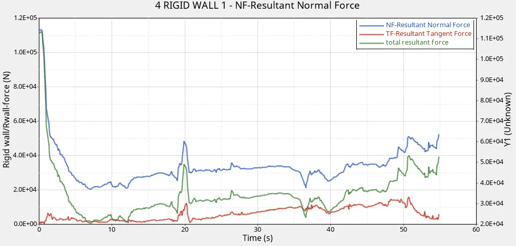
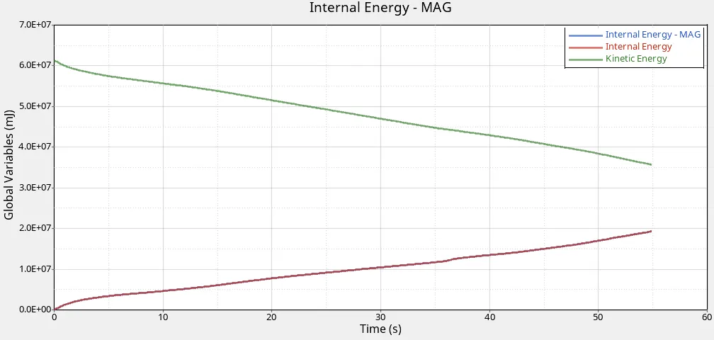
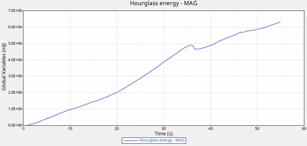
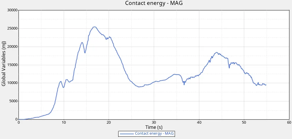
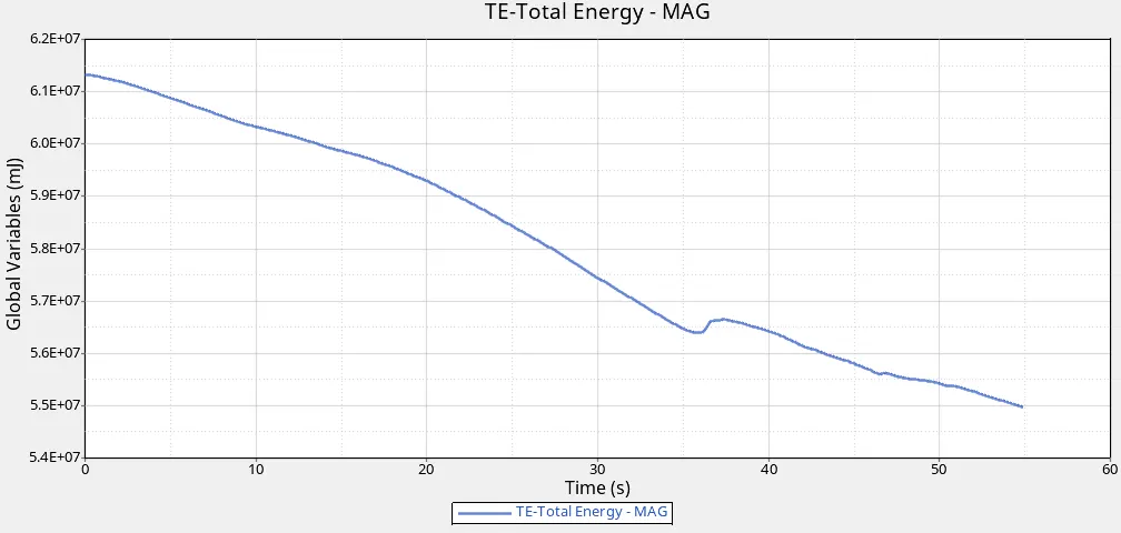
Similarly, when we changed the properties for the model as per give values, we experienced change in results a lot. Like in that case our energy error was fluctuation from 0.0% - (-0.1%) only for all time steps and our mass error was only 0.1659E-03. Here if we observe compared to last result there is huge change in energy error value means results are more stable in this case whereas there was no change observed in mass error value it is same as in earlier case.

And the plots also showed better results.

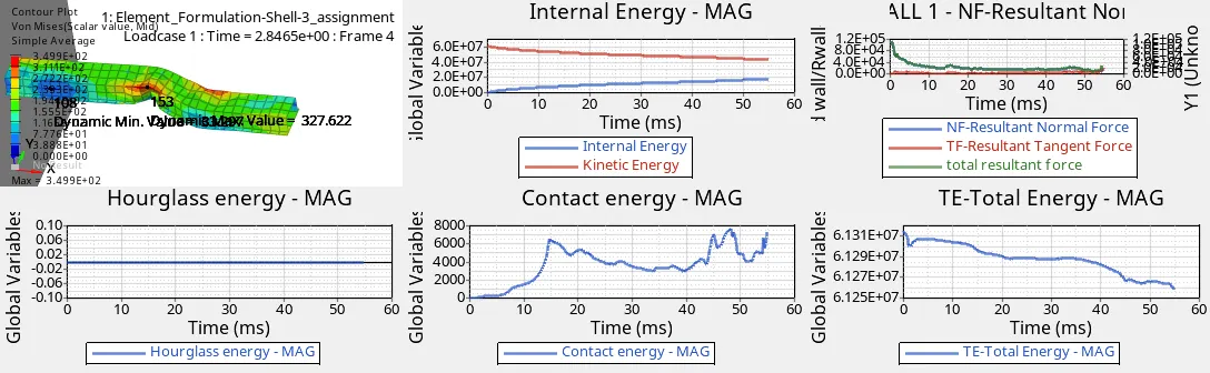
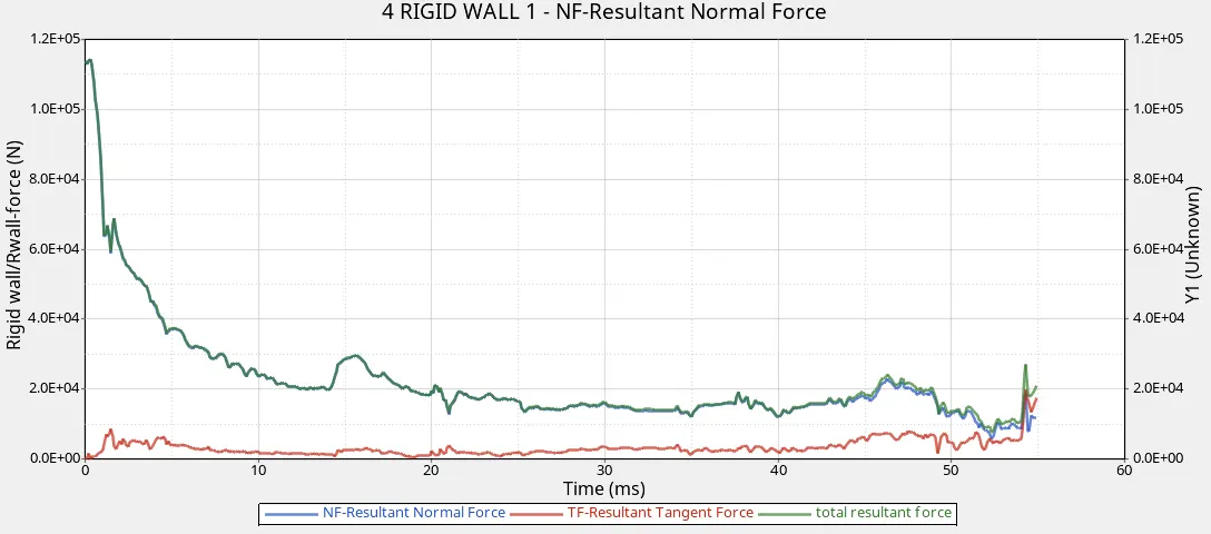
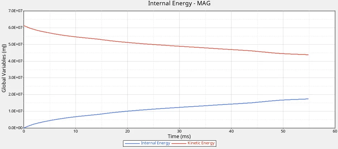
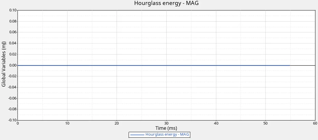
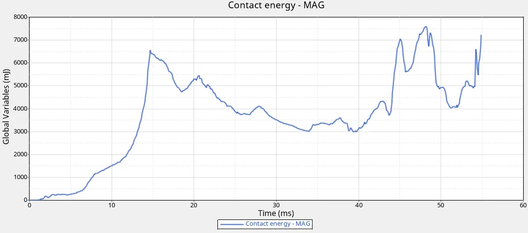
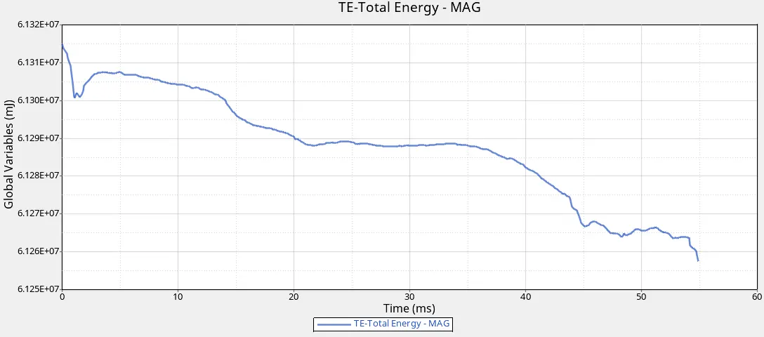
Now if we see both results it was the hour glass energy which was affected the most and may be the reason behind such good results and that may be the reason behind all reasons for all other plots too. So, this raised a question what is this Hourglass Energy.

Hourglass modes are element distortions that have zero strain energy. In these elements, a reduced number of integration points are used to decrease the computation time which causes formation of zero strain energy modes. Hourglass resistance forces are usually either viscous or stiffness related. The viscous forces relate to the rate of displacement or velocity of the elemental nodes, as if the material was a highly viscous fluid. In simple words hourglass means nodes experience deformation but records no stress. So, to correct it we have multiple options.

The choice of hourglass formulation plays an essential role on the quality of results. If the mesh is fine enough, the physical stabilization method can be used. Otherwise, Type 3 and Type 4 formulations are recommended for shell meshes. When the material undergoes elastic-plastic behaviour, the Type 3 formulation is much more efficient. The hourglass coefficient, hm and hf are recommended to be set to 0.1; however, the default value, hf=0.01 can be used for hr.

So, by this information we came to know higher integration points leads to higher stability for solutions. And that can be done by controlling or improving hourglass values which will further improve results and also leads to changes in other values which we can notice in other plots as well.

Now, what were the parameters we changed in property card for this stability in model results.

The last 2 parameters i.e. I_thick and I_plas are used for the results above yield point means plasticity region of material and the other control the things below yield point means elasticity region of material.Now the major out of all was I_shell i.e. 24 as it follows QEPH type which we know stabilises the hourglass energy the most and that too without increasing much cost of solving.

Drive Link :

After changing Properties :

https://drive.google.com/file/d/1PT_HJDlX7XSWsfFpVuYXy5_bpM_h61nD/view?usp=sharing

Without Changing Properties:

https://drive.google.com/file/d/1wtZgYB8cgQxqDRWbx5t0_QRmU57Npggv/view?usp=sharing