Assignment 3-2D Element Formulation Challenge

OBJECTIVE:

Comparison of results with base simulation and improved shell element properties

1.Using the crash beam file from the previous assignment, change the run time to 55 ms.

2. Change the number of animation steps during simulation to a minimum of 25 and a maximum of 60.

3. Run the base simulation without any modification to element properties.

4. At the end of the simulation, do the energy error and mass error checks and determine whether the results would be acceptable.

5. If acceptable, Plot rigid wall forces, internal energy, hourglass energy, contact energy, the total energy of the simulations.

6. Change all the shell elements properties to recommended properties, save this as separate, rad files, and run the simulation.

7. Follow steps 5 and 6.

8. Create a brief report comparing all the results from steps 5 and 6 for both simulations.

9. Comment whether there is any change in the results and why there is any change in the result.

Theory:

Element formulation:

• There are so many elements that we use in radioss to get the desired results. And these elements are categorized by the element formulation technique, which consists of the same elements but varies with respect to some parameters such as type of integration within the element, cost, etc. Based on this element formulation, we can specify the type of elements to be used in our simulation. These are explained below.

In general, there are 3 types of elements. Based on dimensions. They are:

• 1D elements: Which include Springs, Trusses, Beams.
• 2D elements: This includes shell elements like quads(4-noded), Trias(3-noded).
• 3D elements: This includes solid elements such as Tetra, Hexa elements.

2D Element formulation: -

• Before going to the 2D shell element formulation, an important parameter should be discussed. Which is named "Hourglass".

Hourglass:

• "Hourglass is a deformation, that is noticed when an element is deformed due to the applied load. But the strain energy due to this deformation is not recorded for that element". It is also known as "Zero energy deformation modes" where an element is seen as deformed.
• It indicates instability.
• It is also said to be as, non-physical modes of deformation, that occur in reduced or under integrated elements & produce no stress.
• Usually, it can be seen in the post-processing stage, where the elements will have zig-zag formation.
• The elements before & after experiencing the hourglass effect are shown in the below figures.
• Before experiencing the hourglass effect
• After experiencing the hourglass effect

Methods to control the formulation of hour glassing:

There are two methods to control the hourglass effect. They are:

1. Perturbation method (Viscous method)
2. Physical stabilization method (stiffness method)

Procedure:

Case -1 (Without assigning the recommended parameters in the property): -

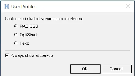
• Initially, after opening the Altair HyperWorks desktop software, the user profile should be selected. And the user profile to be selected is "Radioss" . Because for performing the analysis.

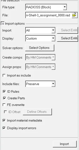
• The next step is to import the given rad file (starter file). This is done by clicking on import, selecting the solver deck in it. After selecting the solver deck, a pop-up appears. In which the given rad file is browsed and by clicking on import, the model with respect to that rad file is imported.

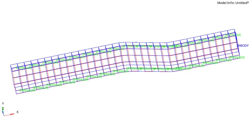
• After importing the model

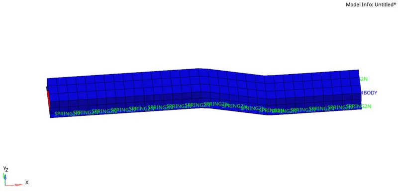
• As the model is in wireframe mode to view it properly, an option named "shaded elements with mesh lines" is enabled. After enabling it, the given model.

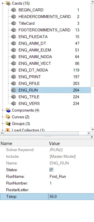
• The next step is to assign the time step value in the card named "ENG_RUN". As mentioned in the question, the run time or time step is 55 ms. This value is entered in the parameter named "Tstop".

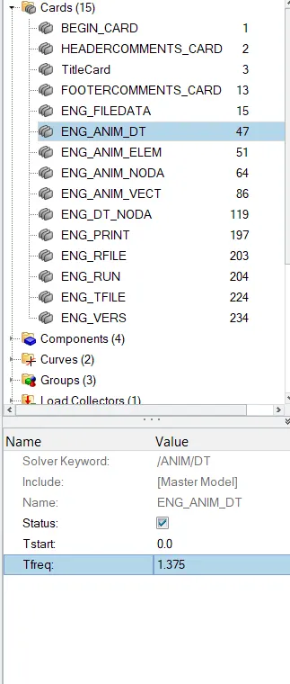
• The next step is to select the number of animation steps required. As mentioned in the question, the number of animation steps can be between 25 to 60. In this challenge, the number of animation steps selected is 40.
• Now to calculate the Tfrequency for a run time as 55 ms with respect to the 50 animation steps.
• The formula used: Tfreq = Time step ÷Number of animation steps

= 55÷40

= 1.375

• Therefore, the Tfreq is 1.375.
• This value is entered in the parameter named "Tfreq" in the card named "ENG_ANIM_DT"

• These values are entered just to perform the simulation.
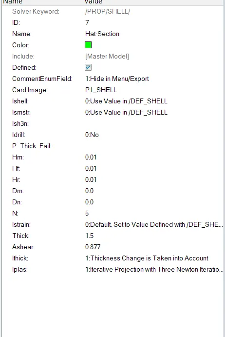
• As in this case, the results are obtained without assigning any properties to the given components. The parameters in the property card are taken the default values.

• The next step is to run the simulation. For doing that, the "radioss" option is used in the "Analysis" panel

• After entering into the radioss panel, initially, the file should be saved in some folder using "save as", and in the options, it is recommended to be written as "-nt 4" as shown in the image below. This means assigning the task to 4 cores in the system, to perform the simulation faster. It depends upon the process of our computer (it has a quad-core processor, then it should be taken as 4. If the system has an octa-core processor, then it is taken as 8). And "nt" means "number of threads". Then click on "Radioss", in order to run the simulation.

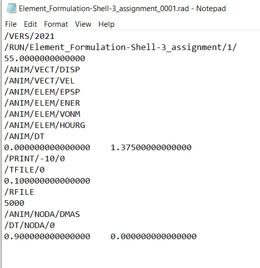
• The next step is to verify the assigned values such as Tfreq, Tstop in the engine rad file (00001.rad) in notepad.

• The next step is to verify the required number of animation files are obtained in the file location that is specified at the beginning. As the specified number of animation steps is 40. The obtained number of animation steps is 41.

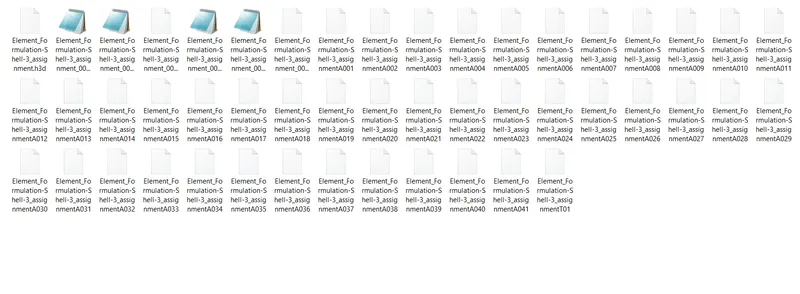
• The next step is to check the obtained values for energy error, internal energy, total energy, mass error from the engine output file (00001.out).

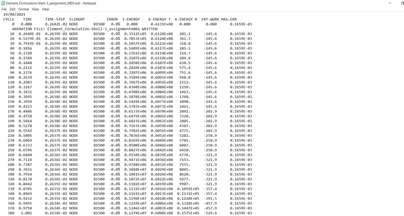
• In the same file, when it is scrolled down to last, the maximum values are seen as shown in the image below. From the figure, the obtained maximum values are energy error: -10.3%, Internal energy: 0.1928E+08 gm^2/s^2, Kinetic energy: 0.3569E+08 gm^2/s^2.

Note: The acceptable tolerance for energy error is -15% to +5%.

• Then click on "results" as shown in the HyperWorks Solver View tab, in order to have a new window. After opening a new window, it automatically switches to HyperView from Hypermesh. It shows to import the h3d file and click on Apply . In order to view the simulation.

• After importing the h3d file, it appears as shown in the image below.

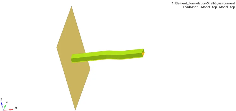
• Then, the next step is to enable the contour. This is done by selecting the contour.

• The next step is to select the various parameters such as the way to view as von-misses, selecting the components, selecting the averaging method, then click on apply at the end

• After applying that, run the simulation. The simulation appears as shown in the below animation.

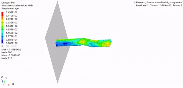
• The next step is post-processing, this is done by obtaining the various graphs for the above simulation. In order to view what is happening within the component (Rail). This is done by switching to Hypergraph 2D .

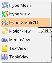
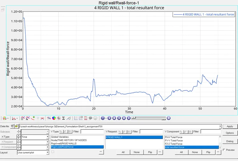
• After switching to the hypergraph 2D, the first graph to be plotted is chosen to obtain the rigid wall forces. So, the various parameters such as the parameter to be on Y-axis (Rigid wall force), the component to be on Y-axis (Total resultant force) which indicates the term be in the graph are chosen and then click on "Apply".
• The obtained rigid wall force graph appears as shown in the image below. The reason for the rigid wall force is dropping from the top is, Initially the rigid wall force acts within the rail component. At that time, the rigid wall force will be maximum, which is indicated as the starting point of the curve. Slowly that force is observed by the adjacent elements, which leads to the decrease of force (results in falling of curve). And this curve again raises up because the rail component is getting contact with the rigid wall. In this way, rigid wall faces fluctuating

• The next step is to plot the graph that indicates some various important parameters such as Internal energy, Kinetic energy, Contact Energy, Total energy, and Hourglass energy. Those parameters are selected and applied from the Hypergraph 2D.

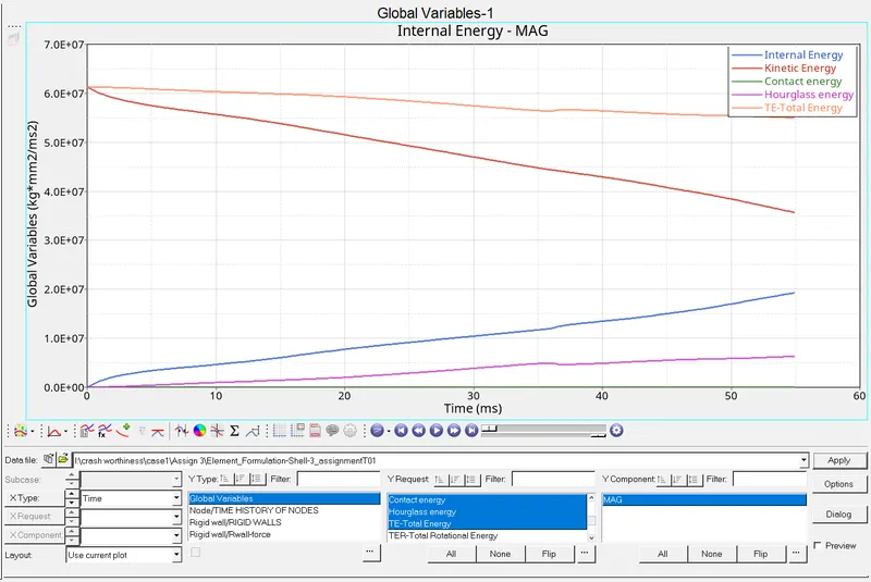
• The obtained graph appears as shown in the image below. The reasons for the behavior of the obtained curves are:

Kinetic energy (KE):

• We know that the formula for kinetic energy is 1÷mv^2
• Since the velocity is applied to the component, there will be a high velocity at the beginning. This velocity decreases with respect to the time, due to the deformation within the rail component.
• So, the kinetic energy is directly proportional to the velocity. That is the reason why, the kinetic energy drops gradually, as shown in the graph below.

Internal energy(U):

• We know that the formula for internal energy is obtained from the first law of thermodynamics. This depicts the change in internal energy is equal to the difference of the heat transfer into the system(Q) and work(W) done by the system.
• Mathematically, U = Q - W
• let us neglect the heat transfer here because the heat transfer is not calculated by the solver (Because Thermal analysis is not done). Now, Work done (W) is the product of force and displacement. The internal energy depends upon the displacement mush here. In the beginning, there is no displacement within the component, that’s why the internal energy starts from zero(origin). when it is subject to acceleration there will be a displacement. As the displacement increases, the internal energy increases, that’s why there is a raise internal energy curve, as shown in the graph below.

Contact Energy:

• The obtained graph for contact energy appears as shown in the graph below. Initially, there will be no contact between the rail component and rigid wall. And also, there is no contact within the component, that’s why the curve starts from origin. And gradually, it reaches the peak because of more contact within the elements of the component due to the deformation. And it drops down as shown in the image below. It raises slowly again to some extent because there will be a contact between the component and the rigid wall. And due to this contact between the wall and the contact takes place, again and again, there will be a regulation in the curve as shown in the graph below.

Hourglass energy:

• As the recommended properties are not specified in this case, there will be a deformation of elements with respect to the strain is not recorded. Which depicts that, the elements undergo an hourglass effect. And there will be no physical stabilization. So, to balance the energy, artificial energy is required. That is hourglass energy. So, there is a lot of hourglass energy needed. So, the hourglass energy starts from the origin and goes on increasing, as shown in the graph below.

Total energy:

• We know that Total energy is the sum of kinetic energy and potential energy. As there is no potential energy plotted here, the kinetic energy is taken into account. The total energy is directly proportional to kinetic energy. As the kinetic energy decreases, the total energy also decreases,

Case 2 (With assigning the recommended parameters in the property): -

• In this case, the properties which are recommended in the question are entered. The procedure is the same as in case-1 till entering the parameters in the property cards. After entering the recommended properties, the property card.

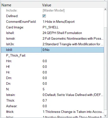
Note: Save this new file in another location. In order to have the entire animation files, engine output files separately with respect to the first case. To compare the results.

• After doing the analysis through the radioss option in the analysis panel, the verification is done to check the required number of animation files are obtained or not.
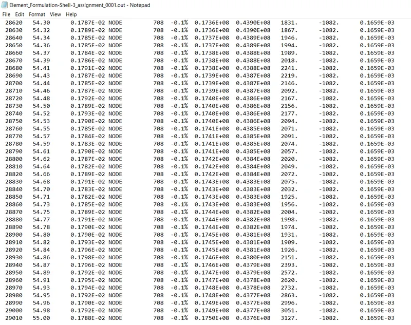
• Then the engine output file is opened to view the various parameters such as kinetic energy, Internal energy, energy error, etc.
• These values are much less when compared to the obtained values in case-1 which depicts the improvement.

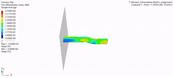
• The obtained simulation, with respect to von-misses view, appears as shown in the animation below.

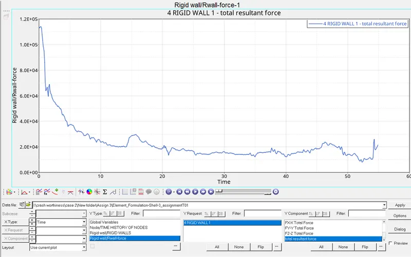
• The next step is post-processing, in this process, various graphs are obtained. In order to see the changes in the result with respect to case-1. The process of obtaining the graphs is the same as in case-1.
• The obtained rigid wall force graph appears as shown in the image below. The graph appears as similar to that of case-1. And there is some improvement in the graph.

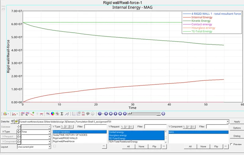
• The next graph consists of parameters such as Internal energy, kinetic energy, contact energy, total energy, Hourglass energy as shown in the image below. The graph seems to be somewhat similar in the aspects of kinetic energy, internal energy. But there will be a small rise in total energy, and the hourglass energy is constant.

Note: The same system of units should be used in all cases.

Comparison between the results of case-1 & case-2: -

Basis for comparison	Case-1	Case-2
Obtained maximum energy error	-10.3%	-0.1%
Obtained maximum kinetic energy	0.3563E+08	0.4376E+08
Obtained maximum Internal energy	0.1932E+08	0.1750E+08
Hourglass energy	Varying hourglass energy	Constant hourglass energy
Reason for hourglass energy	The elements don’t have physical stabilization (Due to the default values in the property cards).	The elements have physical stabilization (Due to the assigning of recommended values in the property cards).
The requirement of hourglass energy	requires hourglass energy to the energy balance.	No hourglass energy is required to balance the energy.
Results	The results are less accurate	The results are accurate

Conclusion:

• Therefore, runner the base simulation and new simulation.
• Compared the results obtained in both cases.
• Finally, I will recommend the same values for the parameters of property cards, to achieve better results.

Learning outcomes:

While performing this challenge, the following aspects are learned:

• Performing the simulation.
• Obtaining the graphs (Post-processing) with respect to that simulations.
• Comparing the obtained values of various parameters such as kinetic energy, Internal energy, Hourglass energy, Total energy, etc.
• Recommending the parameters for the properties to achieve good results.