Assignment 3-2D Element Formulation Challenge

OBJECTIVE:

To compare the results obtained on running the simulation on the crash beam without any modification to element properties and the results obtained after changing the elements properties to recommended properties.

THEORY:

Hourglass Energy:

• When the elements in a model deform but the strain energy is not computed for that deformation then it results in the Hourglass Deformation. It occurs in under integrated elements and produce no stress.
• Reduced Integration can lead to non-physical zero energy modes called hourglass modes.
• Hourglass Formation is controlled using 2 methods,
  • Perturbation method (Q4 Element Formulation): In this method, when Hourglassing is detected an artificial force (defined according to the element stiffness) is applied on the node to stabilize the deformation.
  • Physical Stabilization (QEPH Element Formulation): In this method, the hourglass treatment is done at the material level. This Method is better in terms of cost and accuracy. 

PROCEDURE:

CASE 1:

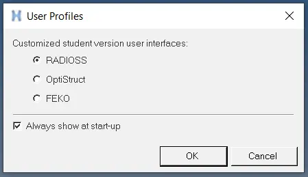
    1. Open HyperWorks and select the user profile as RADIOSS.

                                                      

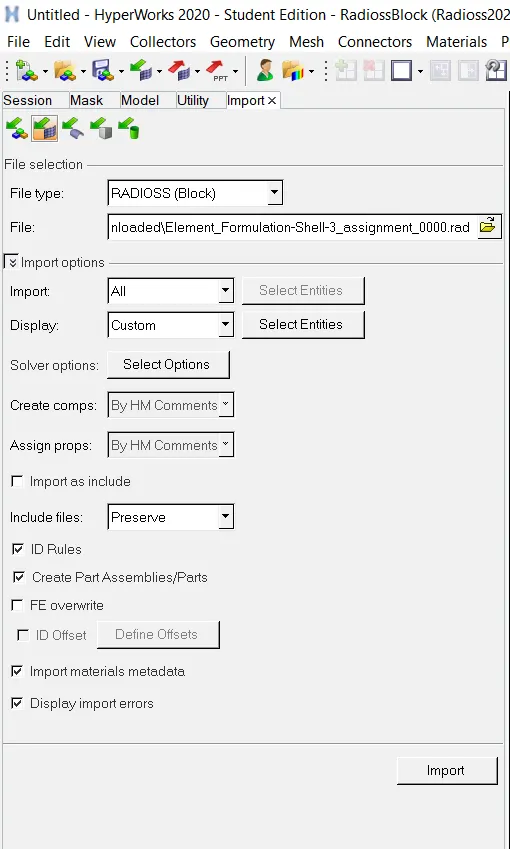
    2. Import the given starter file(file ending with 0000.rad) into HyperWorks using the ‘Import Solver Deck’ Tool.

                                                          

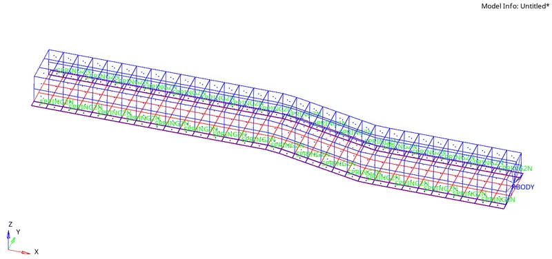
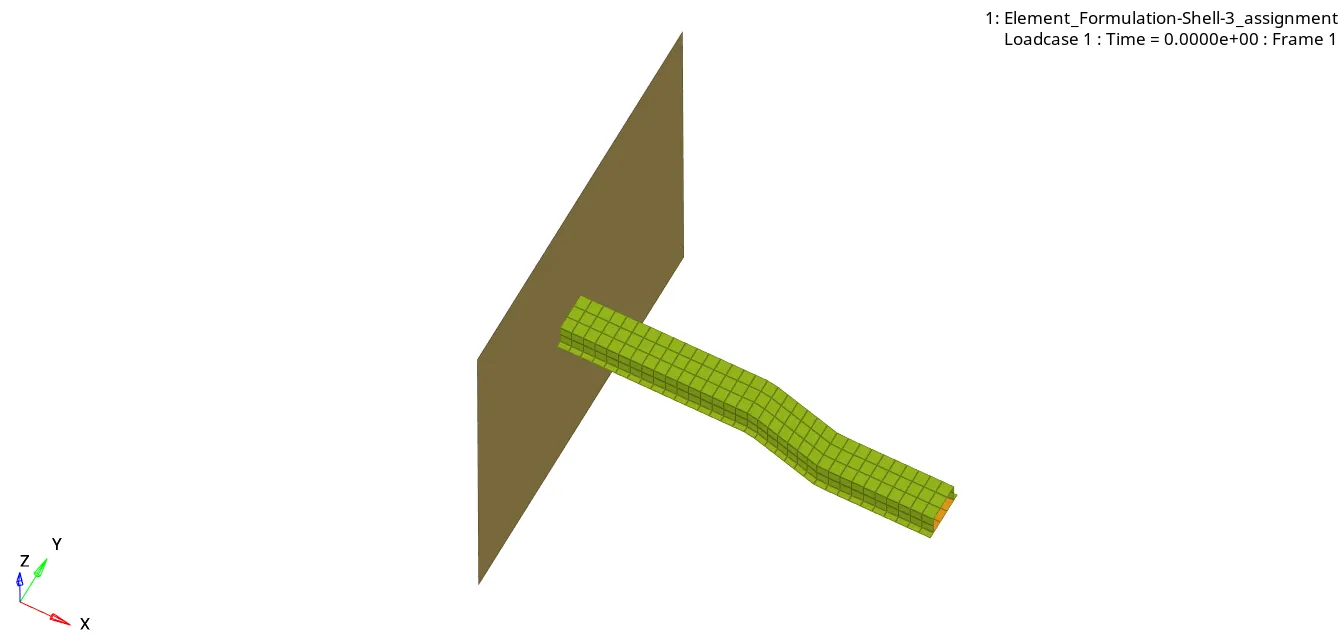
On importing, the model can be viewed in the graphics window.

     

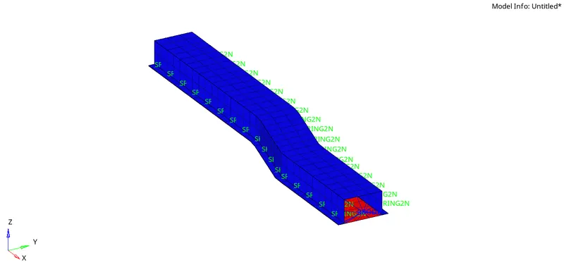
On enabling ‘Shaded Elements and Mesh Lines’ the model can be viewed as shown in the image below.

    

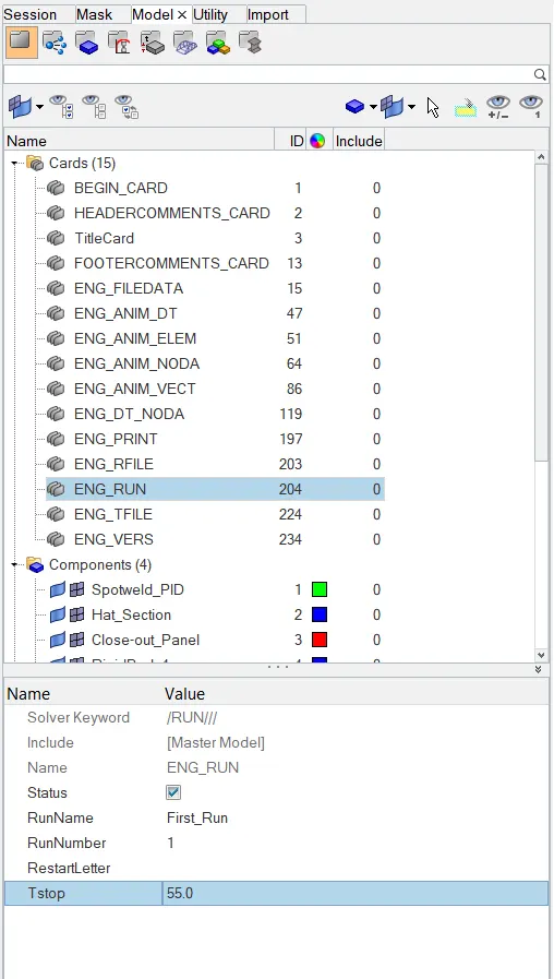
    3. Next, the time step needs to be set to 55 ms. This is done by setting the ‘Tstop’ value to 55.0 under the ‘ENG_RUN’ card.

                                                   

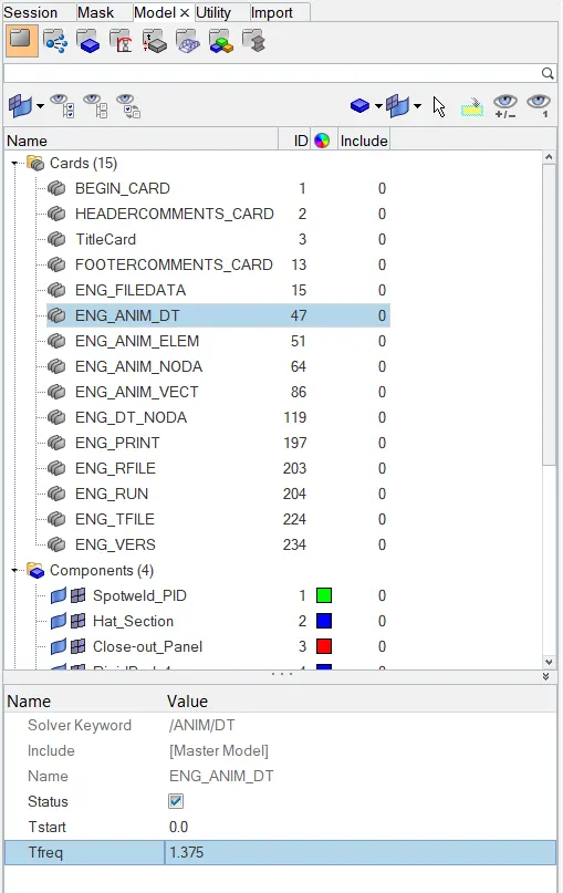
    4. It is specified that the number of animation steps in the simulation can be between 25 to 60. Hence, an approximate middle value of 40 is selected.

To calculate the Tfreq,

Tfreq = `(Timestep)/(Animation steps)` = `55/40` = 1.375

The number of animation steps is set by changing the ‘Tfreq’ value to 1.375 under the ‘ENG_ANIM_DT’ card.

                                                   

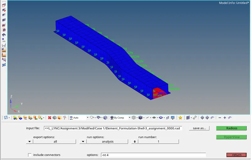
    5. Now the file is run in RADIOSS solver keeping all the values under property card as default, for Case 1.

Analysis > Radioss > click ’save as’ to save the file >export options: ‘all’ > run options: ‘analysis’ > run number: ‘1’ > options: ‘-nt 4’(number of threads set to 4, for faster simulation) > Radioss

          

          

On completion of the simulation, a pop up window opens showing the run summary.

                         

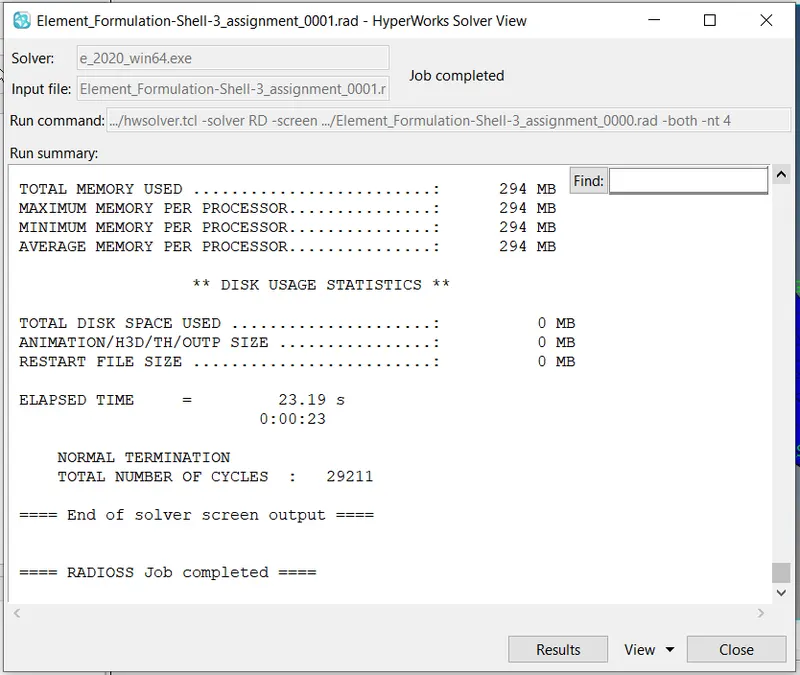
    6. After the simulation is completed, the required values such as ‘Energy error percentage’ and ‘Mass error’ can be viewed by opening the engine output file (file ending with 0001.out) using Notepad.

                             

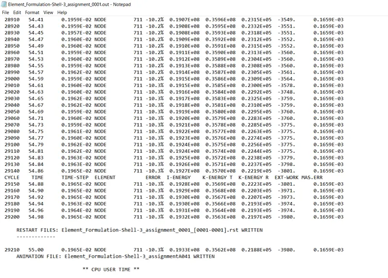
Ideally, the energy error percentage should be at most -15%. Here the value obtained is -10.3% which is within the specified values. Also, the mass error is 0.1659E-03 which is within the acceptable range of 2-4%. Hence the result is acceptable.

    7. To plot the Energy Vs Time graph, HyperGraph is opened. 

Under ‘data file’, the Time History File ( file ending with T01) is loaded.

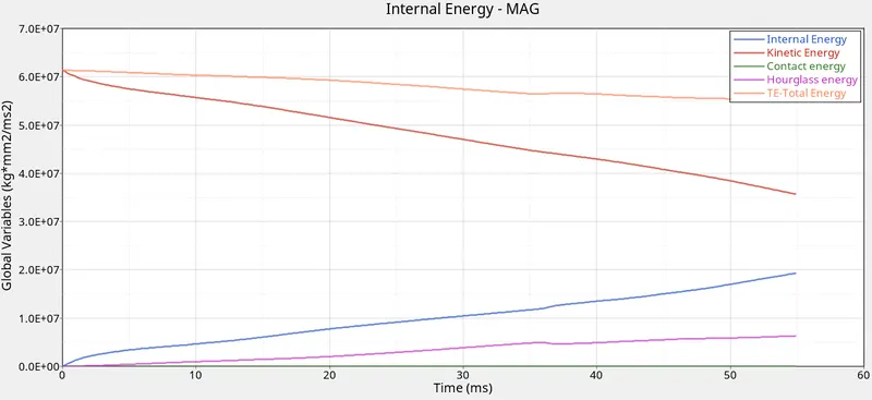
(X Type: Time > Y type: Global Variables > Y Request: Internal Energy, Kinetic Energy, Contact Energy, Hourglass Energy and Total Energy > Y Component: MAG > Apply)

        

All the different forms of energy such as Internal Energy, Kinetic Energy, Contact Energy, Hourglass Energy and Total Energy are plotted.

        

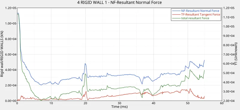
Similarly, the Rigid Wall Forces as a function of Time is also plotted.

        

The Resultant Normal Force, Resultant Tangent Force and the Total resultant force are plotted.

       

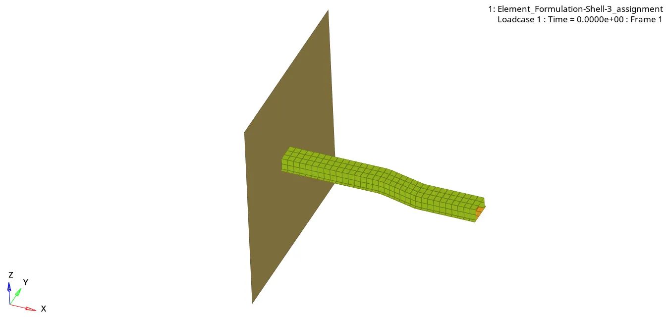
    8. To visualize the simulation results as an animation, HyperView is used. For this, the animation file(file ending with .h3d) is loaded in Hyperview.

        

Animation,

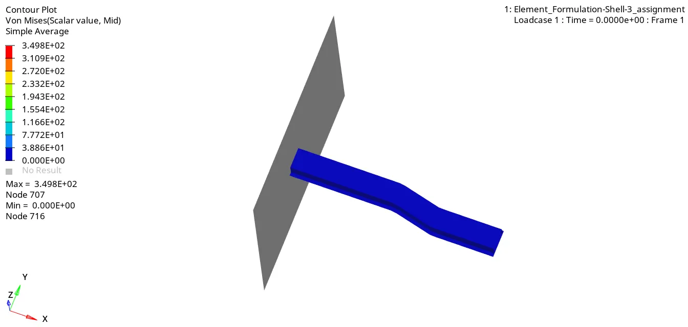
Von-Mises Stress Contour Plot:

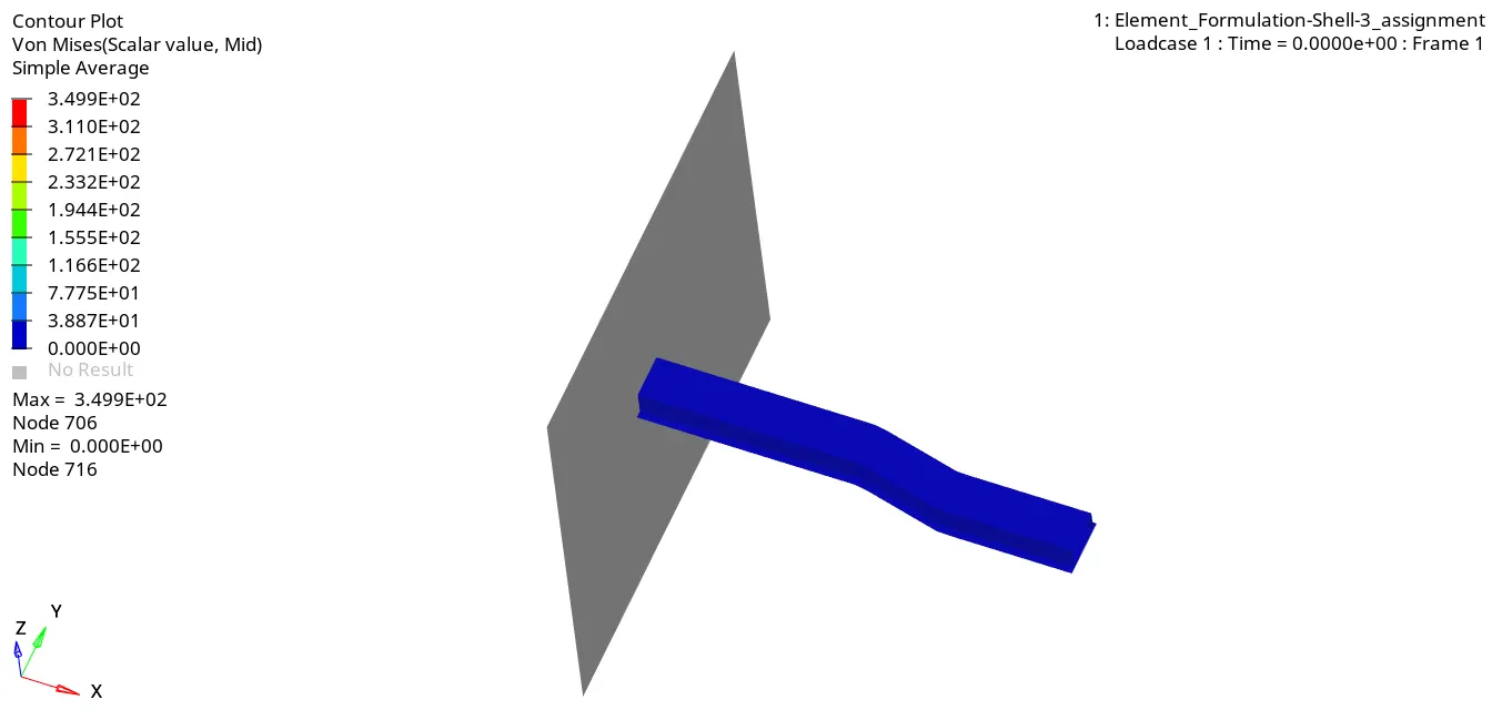
CASE 2:

    1. In Case 2, instead of running the simulation on the default Element Properties they are changed to the required Element Property as specified below,

         

           

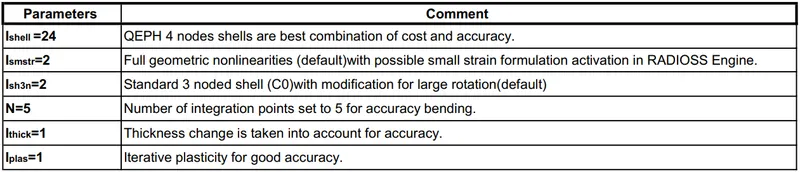
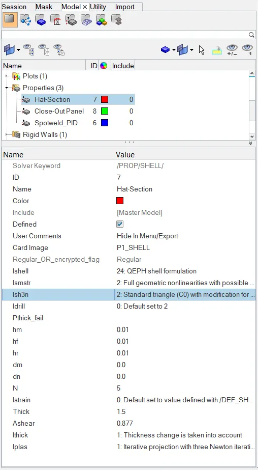
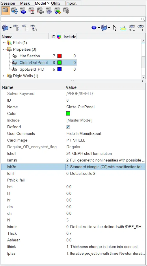
    2. Now the file is run in RADIOSS solver.

On completion of the simulation, a pop up window opens showing the run summary.

                         

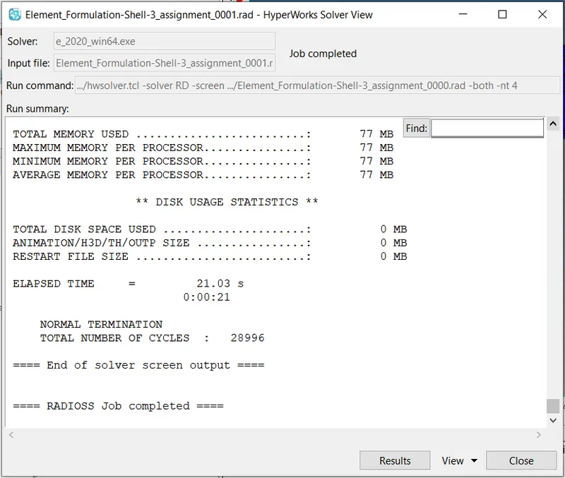
    3. After the simulation is completed, the values such as ‘Energy error percentage’ and ‘Mass error’ is viewed by opening the engine output file (0001.out).

          

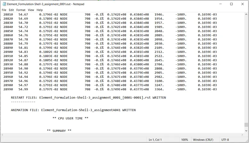
Here the Energy error percentage is -0.1% and the mass error is 0.1659E-03 both of which are within the acceptable range. Hence the result is acceptable.

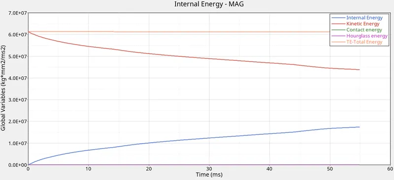
    4. The Energy Vs Time graph is plotted.

         

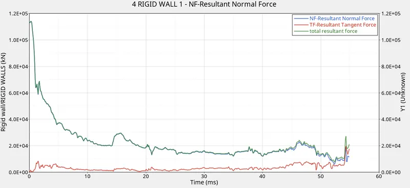
Similarly, the Rigid Wall Force as a function of Time is also plotted.

         

    5. The simulation result is visualized as an animation using HyperView.

Von-Mises Stress Contour Plot:

RESULTS:

Energy Error Percentage and Mass Error:

Case 1:

                

Case 2:

         

Ideally the energy error percentage should be at most -15%. The closer to 0% the better. Here the values obtained for Case 1 is -10.3% and for Case 2 it is -0.1% both of which are within the specified values. Also, the mass error is 0.1659E-03 in both Case 1 and Case 2, which is within the acceptable range of 2-4%. Hence both the results are acceptable. But, due to the use of QEPH element formulation in Case 2, the hourglass formation is controlled and as a result, there is a considerable decrease in the Energy Error Percentage as compared to Case 1.

Energy Vs Time Plot:

 

                                              Fig: Case 1                                                                                                                  Fig: Case 2

Initially, when the velocity is imparted to the elements it is present as Kinetic Energy. But, as the component deforms the Kinetic Energy gets converted to Internal Energy as per the law of conservation of energy. This can be seen in the graph as the Kinetic Energy Curve is falling whereas the Internal Energy Curve is rising.

As the energy is getting converted from one form to another the total energy should remain constant. But in Case 1, due to the presence of Hourglass energy, there is a decrease in the Total Energy. As seen in the graph, when the Hourglass Energy curve rises there is a corresponding fall in the Total Energy Curve.

But, in Case 2 due to the use of QEPH element formulation, the buildup of Hourglass Energy is controlled using Physical Stabilization by adding stiffness at the material level. As a result, the Total Energy remains constant throughout.

Comparison of Energy Values Obtained in Case 1 and Case 2,

                          

Hence, we can see that more accurate results are obtained in Case 2 due to the use of QEPH element formulation.

Rigid Wall Force as a function of Time:

 

                                                   Fig: Case 1                                                                                                             Fig: Case 2

Using the Rigid Wall Force option, the Normal Force, Tangent Force and the Total Resultant force are all plotted. Initially, as the component is in contact with the wall the Normal Force is high but with time it decreases as the Energy gets absorbed.

The Tangent Force(Frictional Force) is zero initially, but with time it increases and fluctuates due to the contact between the component and the wall.

In Case 1 there is a high fluctuation in the forces due to less integration whereas in Case 2 there is a regular drop in the rigid wall forces after the crash.

Animation Files:

 

                                                 Fig: Case 1                                                                                                             Fig: Case 2

CONCLUSION:

In this assignment we learned how to set up a model in HyperWorks and run a basic crash simulation using RADIOSS solver. By repeating the same experiment with 2 different case setups we were able to observe how with the use of QEPH element formulation we were able to control Hourglass Formation and as a result obtain more accurate results.