Assignment 3-2D Element Formulation Challenge

Aim :-

we have to run the simulation on crash beam model with default values in hypermesh and improved recommended properties.

We have to compared the both results and plot the graphs of internal energy, hourglass energy, contact energy and total energy.

Parameters	value	Description
Ishell	24	QEPH 4 nodes shells are best combination of cost and accuracy
Ismstr	2	Full geometric nonlinearities (default)with possible small strain formulation activation in RADIOSS Engine
Ish3n	2	Standard 3 noded shell (C0) with modification for large rotation(default)
N	5	Number of integration points set to 5 for accuracy bending
Ithick	1	Thickness change is considered for accuracy
Iplas	1	Iterative plasticity for good accuracy.

Ans :-

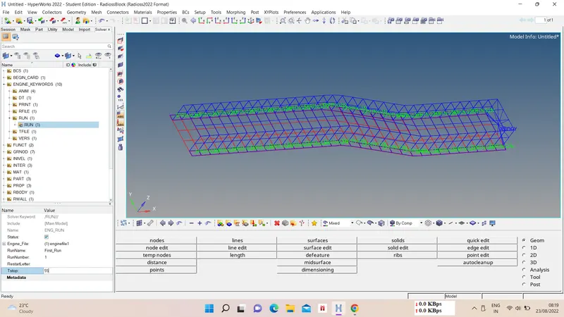
1.Using the crash beam file from the previous assignment, change the run time to 55 ms.

Ans :- First import the model using import solver deck option, select file that ends with 0000.rad file. Now go to solver tab or model tab and change vlaue in engine run tab of Tstop to 55ms.

2. Change the number of animation steps during simulation to a minimum of 25 and maximum of 60.

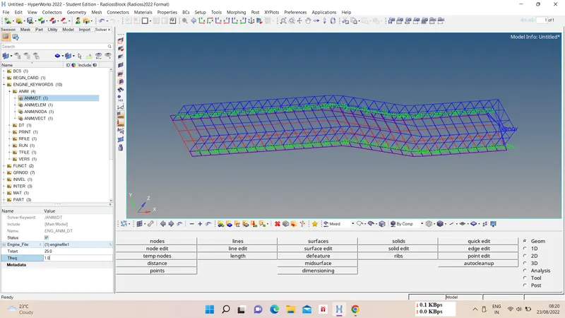
Ans :- Now to change the animation stpes goto solver tab open engine keawords, in that open anim/dt and edit value of Tstart and Tfreq.

3. Run the base simulation without any modification to element properties.

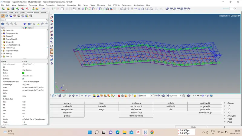
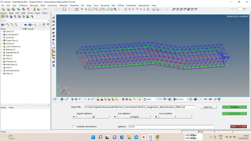
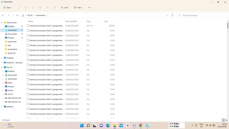
Ans :- Now without doing any modification in properties we have to run the simulation, for that go to analysis - RADIOSS -save file for default values - -nt 4 (for quad core its 4 number of threads) - click on RADIOSS to run the simulation.

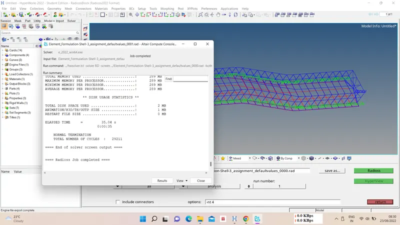
4. At the end of the simulation, do the energy error and mass error checks and determine whether results would be acceptable.

Ans :- Next we have to check the obtained vlaues for energy error for that open engine output file with 00001.out extension.

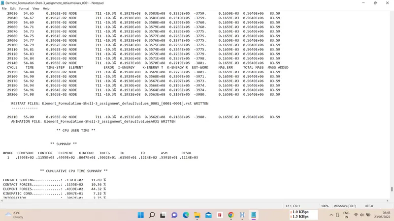
From the image we can see that energy error is -10.3% and acceptable tolerance is -15% to +5%, closer to 0 is the better result.

5. If acceptable, Plot rigid wall forces, internal energy, hourglass energy, contact energy, total energy of the simulations.

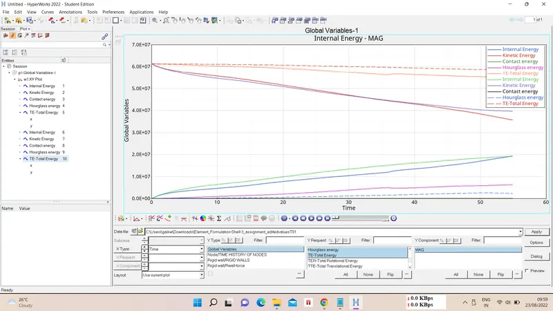
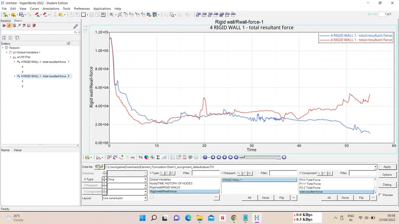
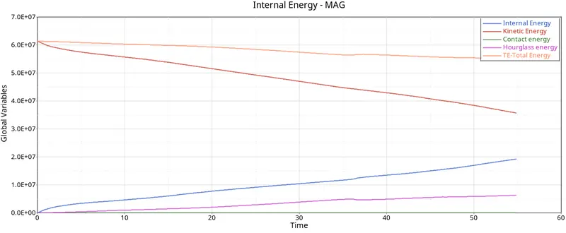
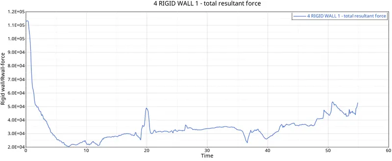
Ans :- As errors are within accepatble range now we can plot the graphs, for that switch to Hypergraph 2D. Now input the file with T01 file name and plot the graph of internal energy, hourglass energy, contact energy, total energy and rigit wall forces.

To visualize the animation simulation, we have to swith to Hyperview. After accessing Hyperview, input the filie with h3d extension and apply it after selection. Now generate the simulation using contour option for displacement contour and Von Mises stress contour.

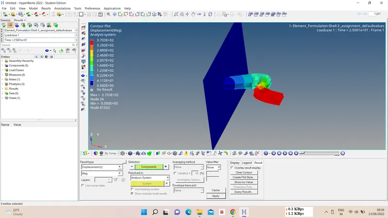
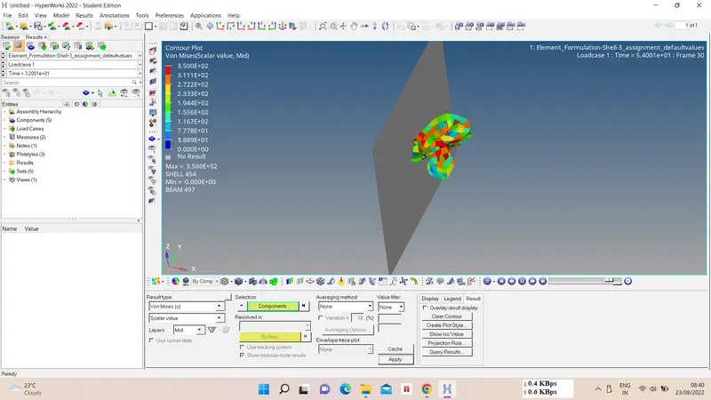
6. Change all the shell elements properties to recommended properties, save this as separate, rad files and run the simulation.

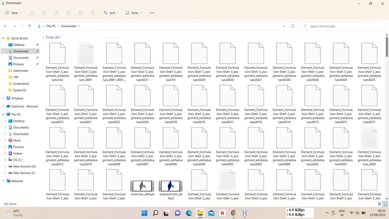
Ans :- Now we have to carry out simulation for new case scenario with given shell element properties. Repeat the 1. and 2. process after importing file into solver deck, after that we have to edit properties for given properties and run the simulation again with store output files.

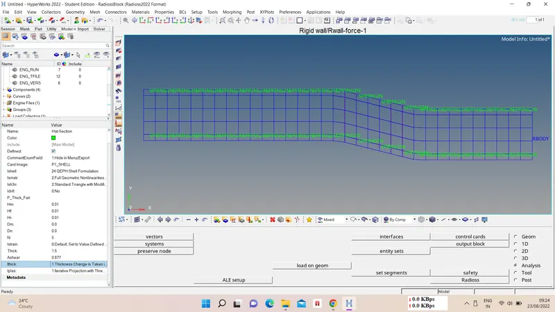
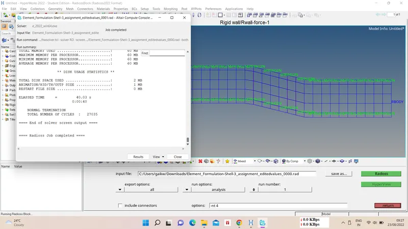
7. Follow steps 5 and 6.

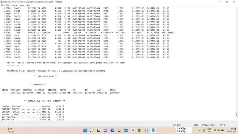
Ans :- We have to follow same steps as before, so using engine ouput file 00001.out we have to check values for energy errors. As we can observe in following image hourglass energy is reduced to -3.8% which is much lower than before vlaue and is closed to zero.

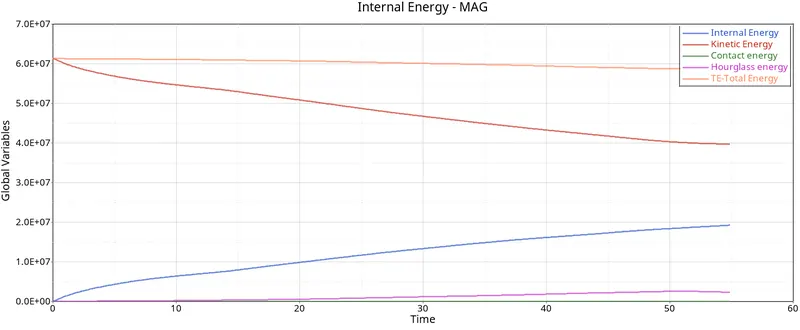
As errors are within accepatble range now we can plot the graphs, for that switch to Hypergraph 2D. Now input the file with T01 file name and plot the graph of internal energy, hourglass energy, contact energy, total energy and rigit wall forces.

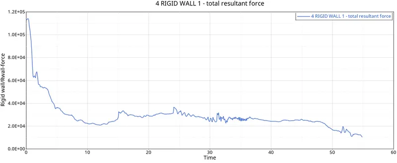
To visualize the animation simulation, we have to swith to Hyperview. After accessing Hyperview, input the filie with h3d extension and apply it after selection. Now generate the simulation using contour option for displacement contour and Von Mises stress contour.

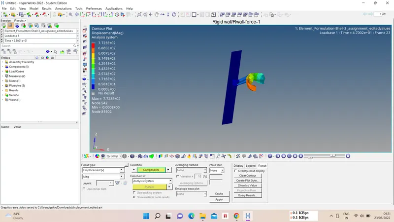
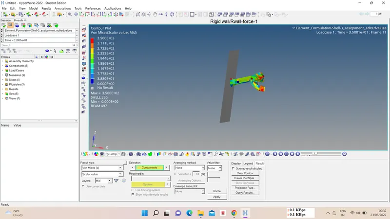
8. Create a brief report comparing all the results from steps 5 and 6 for both simulations.

9. Comment whether there is any change in the results and why there is any change in the result.

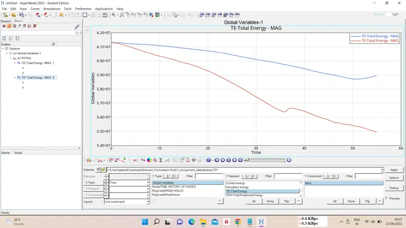
Ans :- We can compare graphs of both cases and can see difference between values behaviour on graph. The obvious difference in both simulations is the reduction in hourglass energy. The introduction of QEPH shell formulation (Ishell= 24) in the second case, provides an artificial stiffness to the shell elements and helps counter hourglass formation.

Talking in more details about both cases differece -

i) Energy Error - As compared to default properties which is -10.3% energy error decreases to -3.8% which is better for recommended properties case.

ii) Hourglass Energy - In default properties case hourglass energy increases with time, in recommended properties case its much near to zero as physical stabilization introduced in it.

iii) Total Energy - Due to increase in hourglass energy total energy is decreased in default porperties case, in second case as there is not much hourglass energy the curve remains much constant.