Assignment 3-2D Element Formulation Challenge

Aim :-

Solve the given model using RADIOSS to show the simulation and graph, and also compare the result with base simulation and improved shell element properties.

The propcess is divided into 2 cases namely;

Case 1 :- Base simulation (Analysis is done based on the given condition)

Case 2 :- Improved Shell Element Properties (Elements properties are changes as prescribed below).

Recommended properties for Case 2:

Parameters		Comment
Ishell =24		QEPH 4 nodes shells are best combination of cost and accuracy.
Ismstr=2		Full geometric nonlinearities (default)with possible small strain formulation activation in RADIOSS Engine.
Ish3n=2		Standard 3 noded shell (C0)with modification for large rotation(default)
N=5		Number of integration points set to 5 for accuracy bending.
Ithick=1		Thickness change is taken into account for accuracy.
Iplas=1		Iterative plasticity for good accuracy.

Case 1 Procedure :-

1. Import the given 0000.rad file by solover deck.

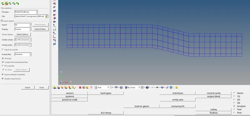
Fig 1 :- Import the model

2. Once the model is imported, change the engine timest ep to 55ms as mentioned in the question, which will be 60ms in given model.

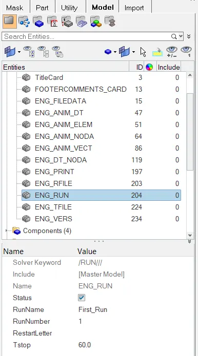
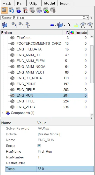
Fig 2.1 :- Given Timestep Fig 2.2 :- Updated Timestep

Also change the animation steps in between 25 to 60,

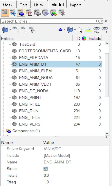
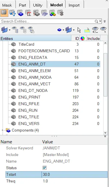
Fig 2.3 :- Given Animation Step Fig 2.4 :- Updated Animation Step

3. Go to Analysis->Radioss and save as the file in a separate folder with .rad extension. Enter "-nt 4" in options which represents number of Threads (nt) and task assigned to 4 cores (4).

Then click on Radioss.

Fig 3.1 :- Analysis Input

The solver starts running, once the analysis is completed check for the window which displays "Radioss Job Completed".

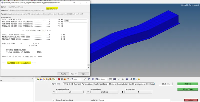
Fig 3.2 :- Analysis Completed for Case 1

4. Check for Energy errors & Mass error by opening the 0001.out file in notepad. Energy error in between -15% to +5% is acceptable.

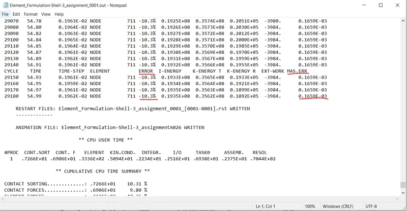
Fig 4 :- Solver Output data for Case 1

5. Open Hyperview or click on "results" in the solver view tab. It automatically enters the h3d file for simulation, then click on apply.

Fig 5.1 :- Hyperview Input

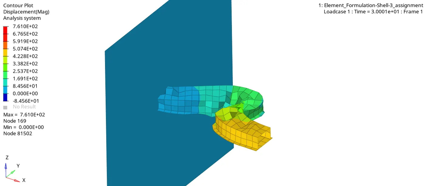
Fig 5.2 :- Displacement Analysis for Case 1

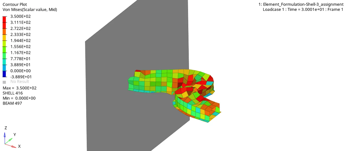
Fig 5.3 :- Von Mises Analysis for Case 1

6. Generate a graph representing chnage in internal energy, kinetic energy, hour glass energy & TE-total energy by slecting as shown below,

Fig 6.1 :- Hypergraph Creation for Case 1

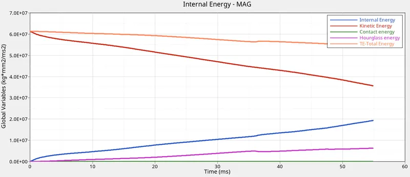
Fig 6.2 :- Change in Energy Representation for Case 1

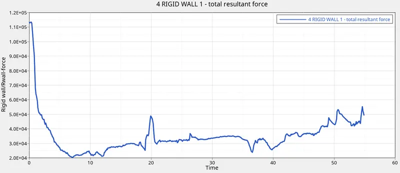
Fig 6.3 :- Total Resultant Force for Case 1

Case 2 Procedure :-

1. Procedure 1 & 2 mentioned in Case 1 is to be repeated for Case 2.

2. Chnage the element properties as defined in the problem.

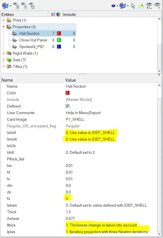
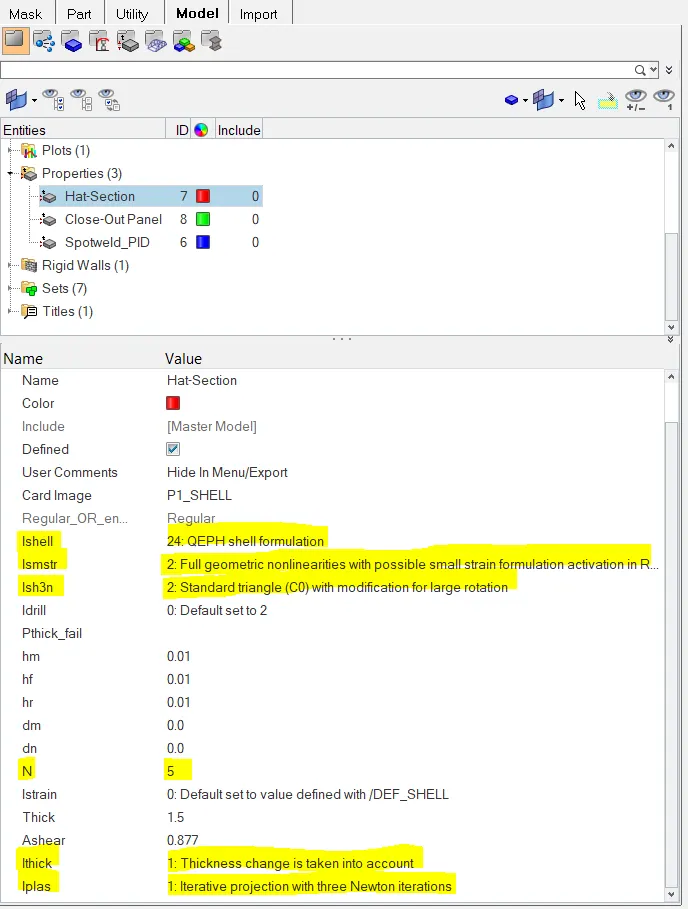
Fig 7.1 :- Existing Element Property Fig 7.2 :- Updated Element Property

2. Now run the Radioss analysis as mentioned in Case 1->step 3. And view the resluts in 0001.out file.

Energy error is reduced to -3.3% which is acceptable.

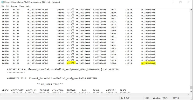
Fig 8 :- Solver Output data for Case 2

3. Switch to hyperview to run the simulation. follow the same steps as in Case 1.

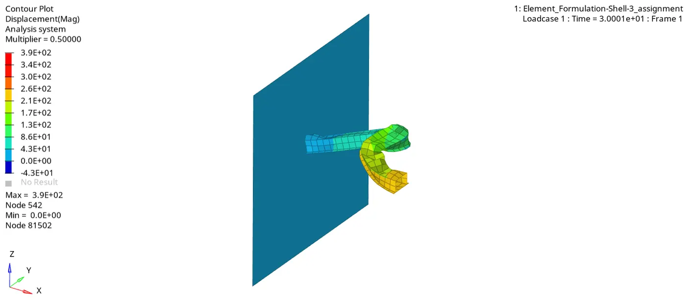
Fig 9.1 :- Displacement Analysis for Case 2

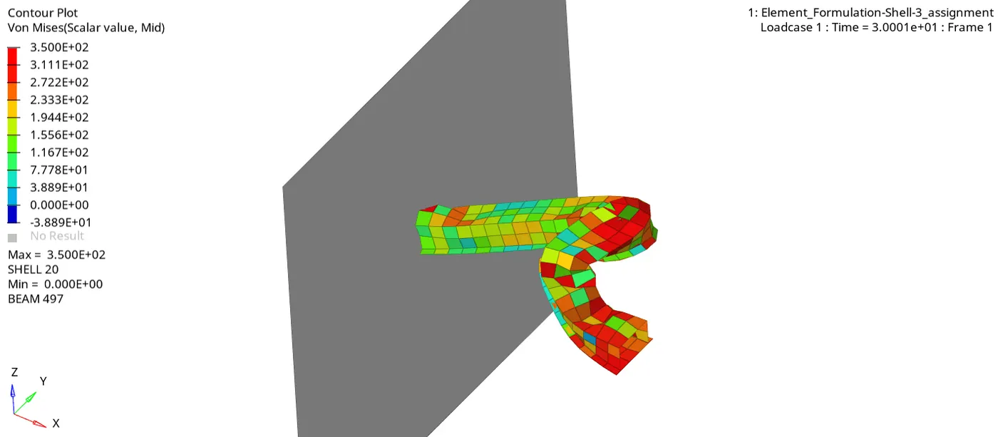
Fig 9.2 :- Von Mises Analysis for Case 2

4. Generate change in energy and total resultant graphs similar to Case 1.

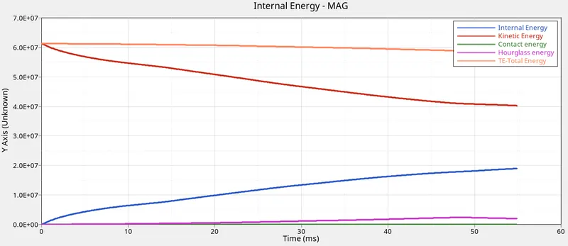
Fig 10.1 :- Change in Energy Representation for Case 2

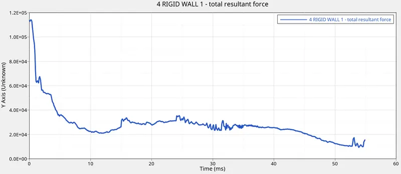
Fig 10.2 :- Total Resultant Force for Case 2

5. Compare both the results by graphical representation,

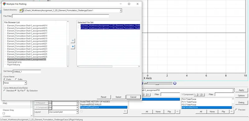
Fig 11.1 :- Combining the results

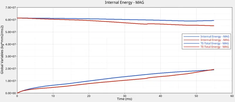
Fig 11.2 :- Change in Energy Graph Combined

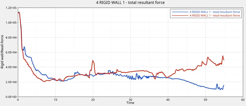
Fig 11.3 :- Total Resultant Force Graph Combined

Observation :-

1. Internal energy and contact energy in constant in both Case 1 & 2.
2. Rigid wall force decreases in both the cases.
3. Total energy will decrease in Case 1 and increase in case 2.
4. Hourglass energy will increase in Case 1 & constant in Case 2.

Result :-

The analysis is carried out in 2 different cases using Radioss, simulated for change in displacement & Von Mises stress using Hyperview, represented change in energy and rigid wall resultant force results using Hypergraph 2D.