Assignment 3-2D Element Formulation Challenge

OBJECTIVE: To solve the simple crash model using Radioss and extract the results of simulation using Hyperview and Hypergraph and also compare the result with element formulation Q24 and with out element formulation.

Procedure

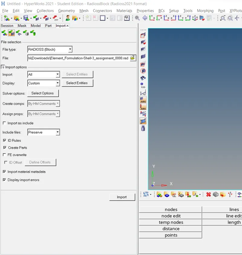
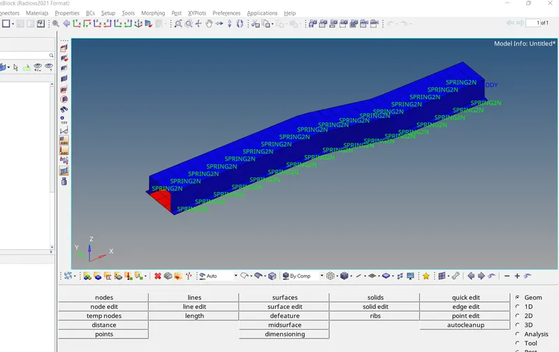
Step 1: Import the .rad file using import solver deck option. Here before importing the .rad file first select the solver as Radioss

Step 2: Modification of run time and plot frequency

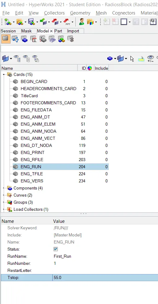
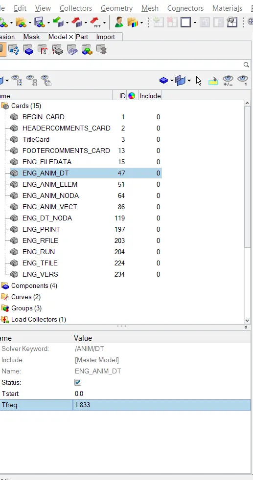
The run-time can be changed from 60 to 55ms by altering the value in the ENG RUN control card. The output time step has been chosen to give 30 animation steps. Therefore the frequency

Tfreq=55/30 = 1.833.

STEP 3: Run the base simulation without any modification to element properties

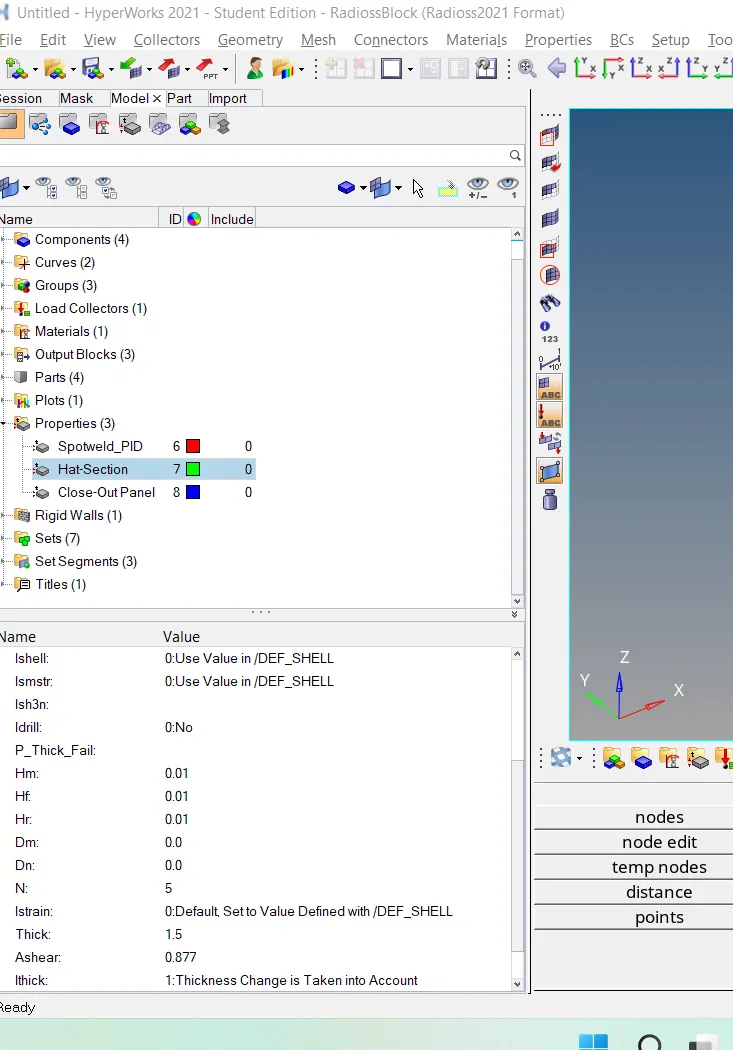
For this, we can go to the Analysis >> RADIOSS and in the next section, we are given the option to save the file before running it in the solver. We can go ahead and give it a different name from the base file to avoid confusion. Clicking save as! It creates a new folder and saves all the output files.

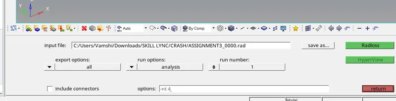
n the Option -nt 4- that is number of threads to make simulation faster. Then run the analysis using radioss option. After completing the analysis the .OUT file can be viewed to check energy error and mass error are within acceptable range.

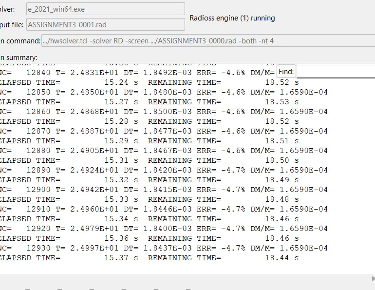
Step 4: Now check the end of solver where there will be error percentage and for this model error percentage is -4.6% and which satisfies the ideal condition i.e, less than -15%. Here negative sign indicates energy is dissipated, the reason of dissipation of energy is discussed in results. Now simulation model is accepted

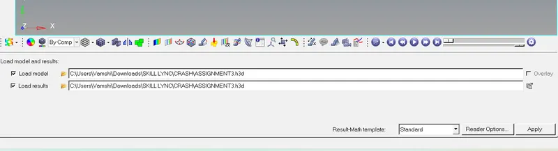
Switching to Hyperview

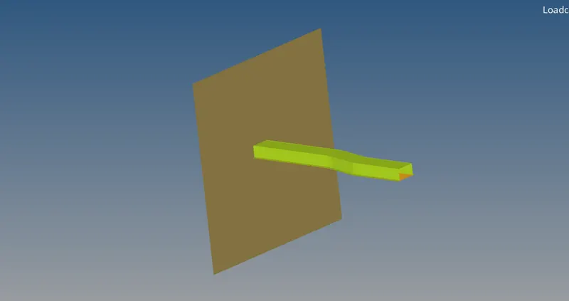
• After accessing Hyperview, we should input the simulation file. For this, use h3d file that was generated when RADIOSS processed the starter file. It is generated in the files swhich are shown in the picture above. After selecting it, we can click 'apply

Using Hypergraph to plot energy and force graphs:

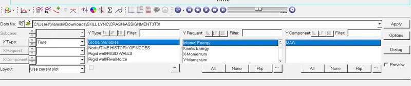
• To plot various graphs by using the results obtained, open HyperGraph 2D from the drop down menu.

Since the TO1 file contains all the time based data obtained from the simulation, select the TO1 file to open

Energy plot of without element formulation:

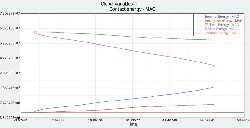
From above plot we can see that hourglass energy dissipation is more and now reason behind the more error negative percentage in solver is this, more artfical enrgy is created i.e, hourglass enegy in order to integrate the shell elements and due to more hourglass energy there is rise in total energy.

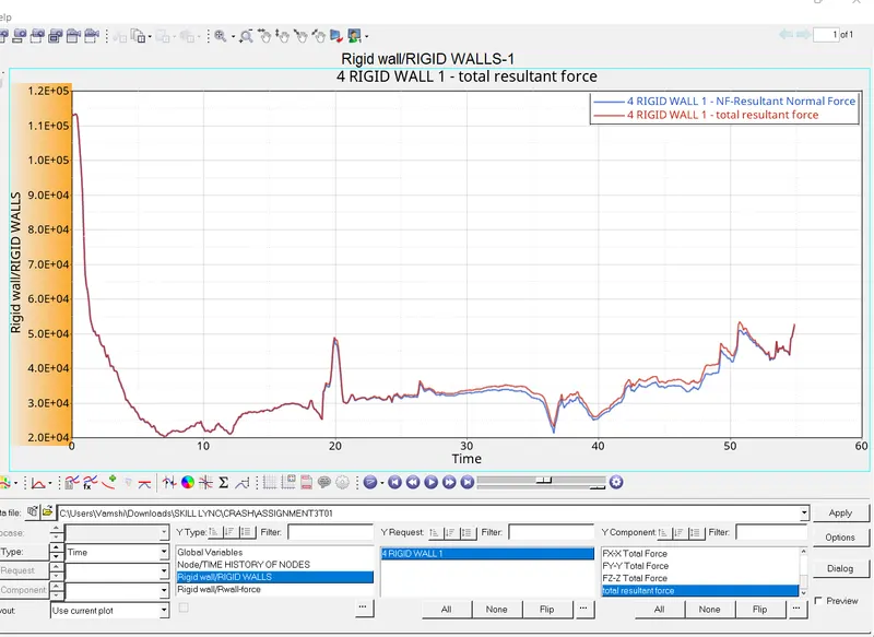
PLOT WITH RIGID WALL FORCES

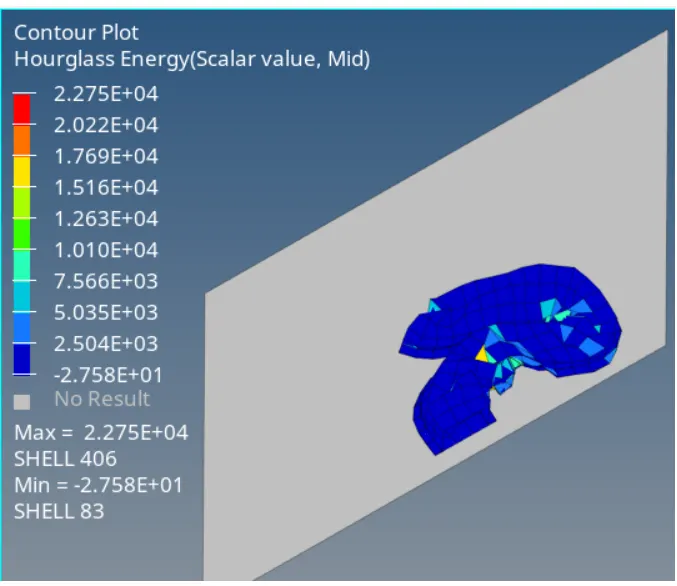
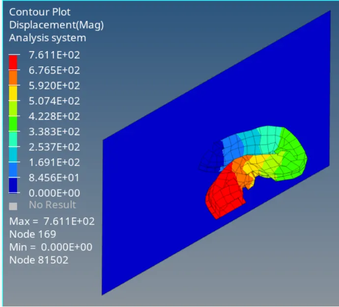
When recomended properties are changed from the base values, simulation results shows that

1. Total Energy remains constant rather than decreasing which is clear from the energy error which went till-4.7% now changed to -0.1%.

2. Hourglass energy which was increasing changed to zero throughout the simulation.

3. Contact energy characteristics are same in both cases.

4. Internal energy is having a gradual increasing characteristics in both the cases. 5. Rigid wall forces also decreased to a lower value than that of default value rigid wall force value.

6. Contour plots shows that there is a slight increase in maximum displacement of element with recommended property values.

Hourglass energy:

• In FEA, the hourglass mode is also known as the "zero energy mode" because deformation energy of elements under hourglassing mode is zero. But the hourglass energy is not equal to zero.

. In a shell element which have a number of integration points, for reduced computation effort, a reduced integration which uses a single integration point is used. In such cases, the deformation mode from the analysis results will be false. This is called hourglass phenomenon.

. This is just a non physical zero energy mode which leads to excessive element distortions. The more structured and less distorted your elements are, the better the results.

To solve this problem,

1. Mesh Refining is a solution. Hourglassing is more prone in coarse mesh.

2. Fully Integrated elements are better though computational time increases vastly and fully integrated elements are prone

3. Providing a small arbitrary stiffness in the mode in which hourglass deforms. This is only a FEA point of view and in actual physical system,

there is no such stiffness. This is what is called as Built in hourglass controls.

4. Viscous damping