Assignment 3-2D Element Formulation Challenge

AIM: To get a view of the properties of the 2d shell elements and also to,Compare the results with the default propertiy cards with the improved shell element properties

here , we do it in a case wise lets say CASE1 with the default and CASE2 with the modified one

CASE1:

• import the model from the solver deck
• change the view and check all the things in the model tree

for the case1 and case2 we will be we have to change the Tstart,Tstop values

• go to cards in the model tree, and drop down to sub trees
• go to>ENG_RUN>, change to Tsop as 55
• go to >ENG_ANIM_DT> and load the Tstsrt value as 25
• these are visible at the section down the database

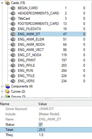
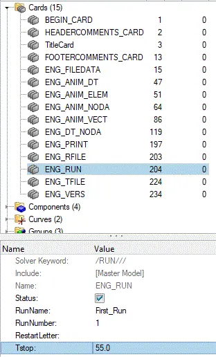
CASE 1 PROCESS:

• as all the requisites for the analysis are set in we just have to check and run the RADIOSS
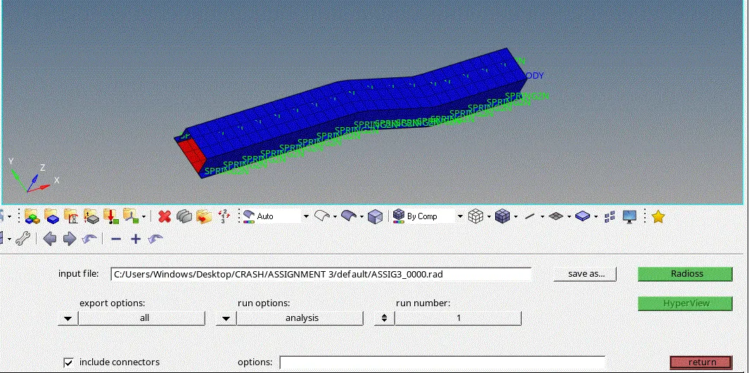
• GO to ANALYSIS > there we can see various set up commands
• choose the radioss, it leads to the radios run commands
• SET the destination file location and save it as .rad files
• set export options as all, this is because of the any of the commands are off, it will be included while eporting or running
• click the INCLUDE CONNECTORS

HYPERVIEW:

• Once the commanda are given , run the radioss

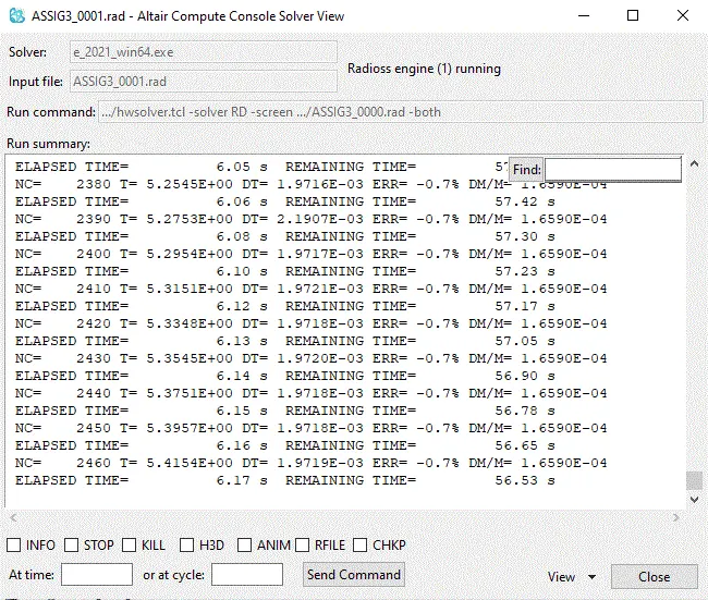
• radioss solver appears, performing the operation, if all the preprocessig is correct radios, shows zero errors and complets the run
• results are to be viewed on hyper view , as clicking on results directly leads to the hyperview

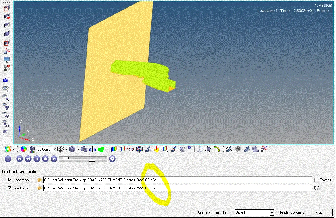
• there are certian file locations in .h3d format which is previously set in with our results, also we could change the name and file location
• this file is the combination of all the ANNIMATION files
• we could play the animation,of our crash analysis
• as we have to analysis results of various, stress and displacements that occur in the analysis go to CONTOUR

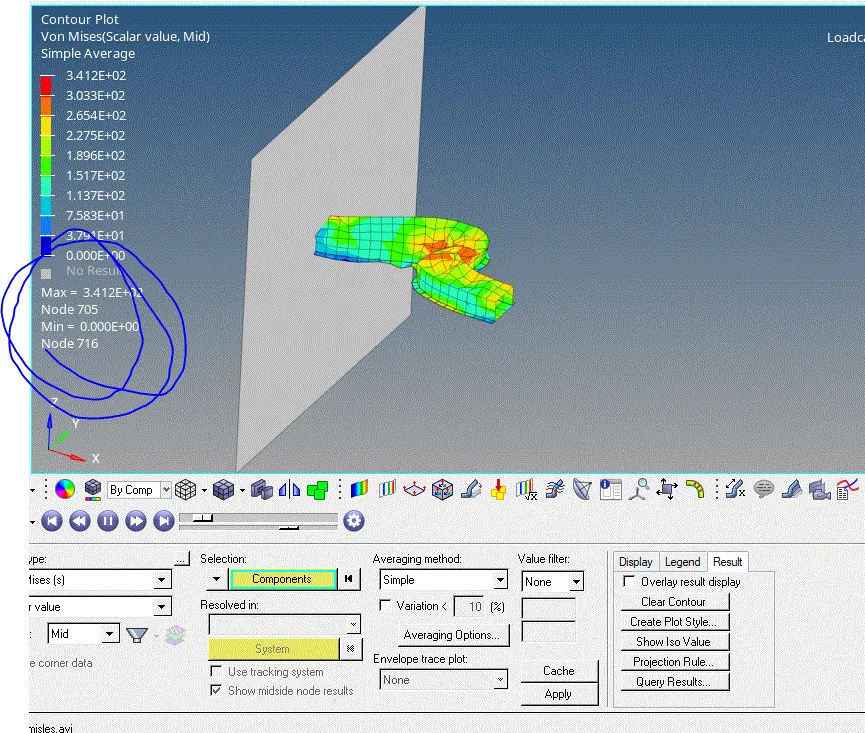
• Select the result type, averaving method and all other required option for the related result type
• with change change in resilt type, we could see the change in colour which represnts the related results
• lets see the results for the VON-MISSLES stress , see the change in the colour representation and note the maxium values

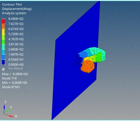
• simillarly extract the results for displacement and others

hypergraph:

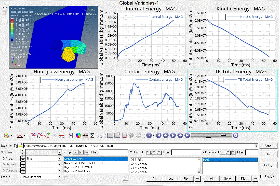
• we have to plot the graphs of the extraced results in order to understant the behaviour of the analysis
• inorder to plot the graphs, split the tab and set the secondary ta in hyper graph mode
• load the T01 file , which will be in t same location , with our 0000.rad files

• this T01 are the hypergraph plot point files
• once the files are selected,set the necessary plot options and apply , a 2d graphical enterface aoopears with the curves plotedin note the values for the further comparasion
• we can split the interface , with as many plots as we requird

CASE2:

In this case we have to change the shell element properties,as given

Parameters		Comment
Ishell =24		QEPH 4 nodes shells are best combination of cost and accuracy.
Ismstr=2		Full geometric nonlinearities (default)with possible small strain formulation activation in RADIOSS Engine.
Ish3n=2		Standard 3 noded shell (C0)with modification for large rotation(default)
N=5		Number of integration points set to 5 for accuracy bending.
Ithick=1		Thickness change is taken into account for accuracy.
Iplas=1		Iterative plasticity for good accuracy.

• the procedure is as same as the above , we are just comparing the results between the default and modified shell element properties

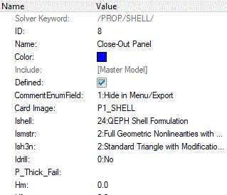
• all the preprocessing and set up that we have followed for the default one are the same with the current one
• lets see the after results plots of the modified properties

hyperview:

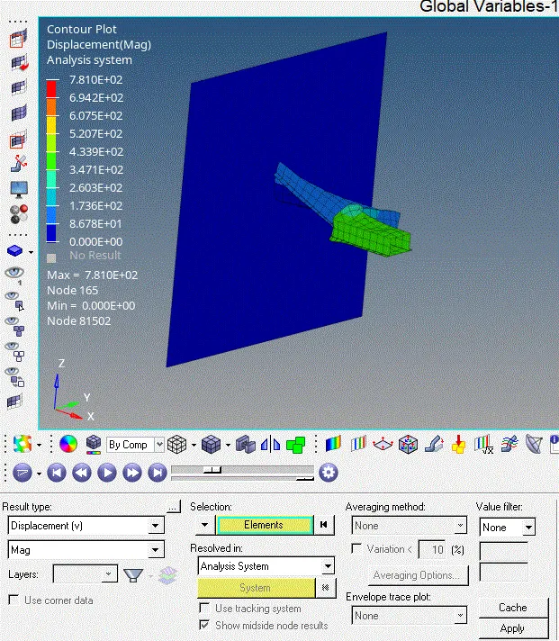
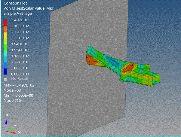
• we can clearly see the the change in ammout of deformation even visible, with the new properties
• even the crashing chages, at the wall all the plots, annimations are as shown

hypergraph:'

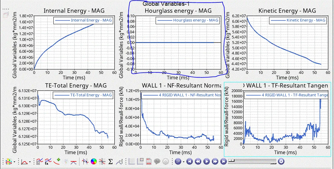
• all the necessary graphs are plotted with various input relations
• these axis coordinates are nothing but the, required results types
• global varoables and rigid wall forces are plotted as shown

RESULTS:

• as we have changed, the shell properties we could clarly see the changes in the results
• there is a little increase in the displacements in case2 than in case1
• as we have induced reduced integration schemes which avoids the ou glass , we can notice that hour glass energy becomes zero in case2
• all these plots files are stored as report in .itp format
• we could directly access these grapgs from these files