Assignment 11

Discretization : The numerical solution of differential equations cannot produce a continuous distribution of the variables over the solution domain, thus the aim instead becomes to produce a set of discrete values at a number of nodes that cover the solution domain. There are three popular methods to discretize

1. FDM ( Finite Difference Method ) 2. FEM ( Finite Element Method ) 3. FVM ( Finite Volume Method ).

All have them have there advantages and disadvantages and user should consider them for solving their particular simulation.

Discretization length effects the time-step when explicit solver is used.

Explicit method :

In the explicit method, the value of pressure, temperature, etc. at the new time is based on the values of only the subvolume in question and its neighbors. The calculation is direct and does not require iteration. To ensure numerical stability, the time step must be restricted to satisfy the Courant condition. This makes the explicit method undesirable for simulations that are relatively long (on the order of minutes). This method will produce more accurate predictions of pressure pulsations that occur in engine air flows and fuel injection systems.

• The relation between the time step and the discretization length is determined by the Courant number, when the explicit solver is used. Courant condition is given below :
• `(Δt)/(Δx) *(|u|+c) <=0.8*m`
• ∆t = time step (s) ; ∆x = minimum discretized element length (m)
  u = fluid velocity (m/s) ; c = speed of sound (m/s)
• In present analysis courant no. should be less than 0.8. Care should be taken that as ∆t ∝ ∆x, the discretized element length shouldn't be unnecessarily small as it increases the time step.
• To ensure above disparity doesn't happen there's a general rule used in GT-suite that for intake system, discretization length ≈ 0.4 x bore-dia of cylinder and for exhaust-system ≈ 0.55 x bore-dia of cylinder. The exhuast has higher discretization length owing to higher velocity of flue gases.
• For SI-engines operating at >6000 RPM discretization length should be much decreases to capture proper wave-dynamics of the engine.

1. CASE STUDY (Varying discretizing length) ON CI ENGINE (single-cylinder) :

• The study is done on this single-cylinder diesel engine

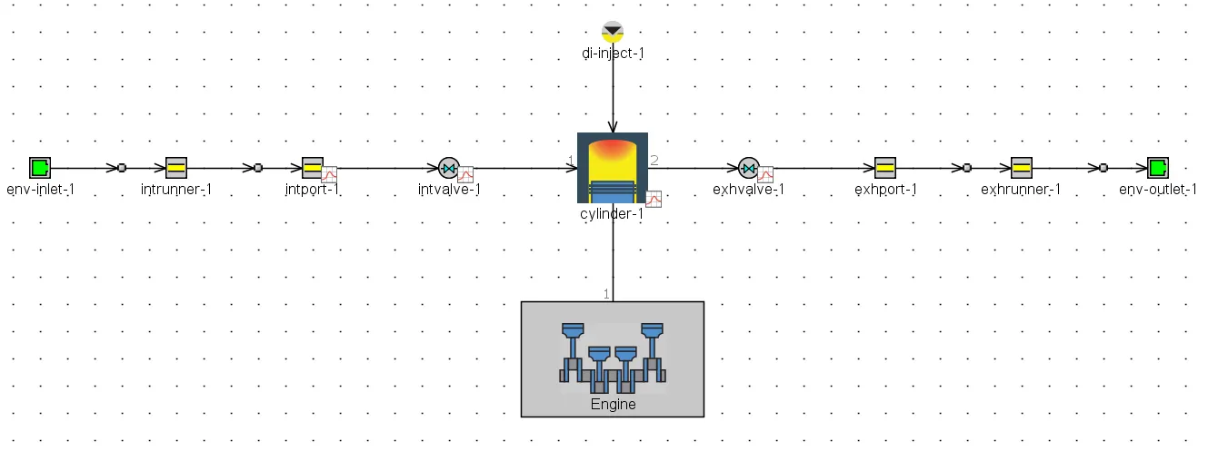
Discretization Length:

• Approximate length of each sub-volume where solution quantities (pressure, temperature, mass fractions, etc.) are calculated.
• The discretization length does not need to be an even fraction of the entire pipe length; the code will adjust to divide the pipe appropriately into an integer number of sub-volumes. The discretization length will affect the time step when the explicit flow solver is used.
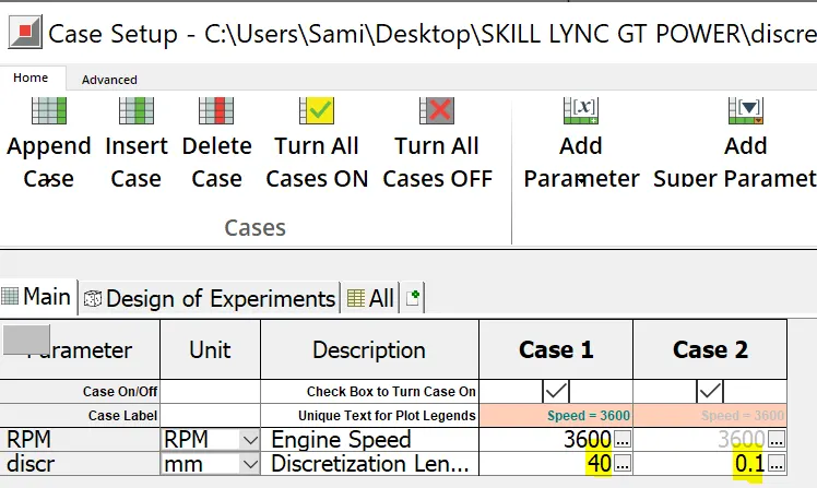
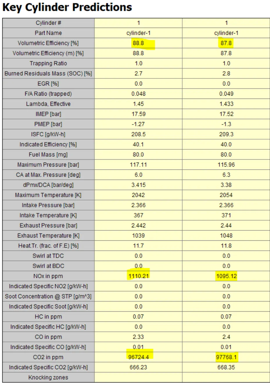
• The case setup is set for two discretziing lengths i.e. 40mm, 0.1mm. to study how results and time taken for simulation are effected.

Case setup :

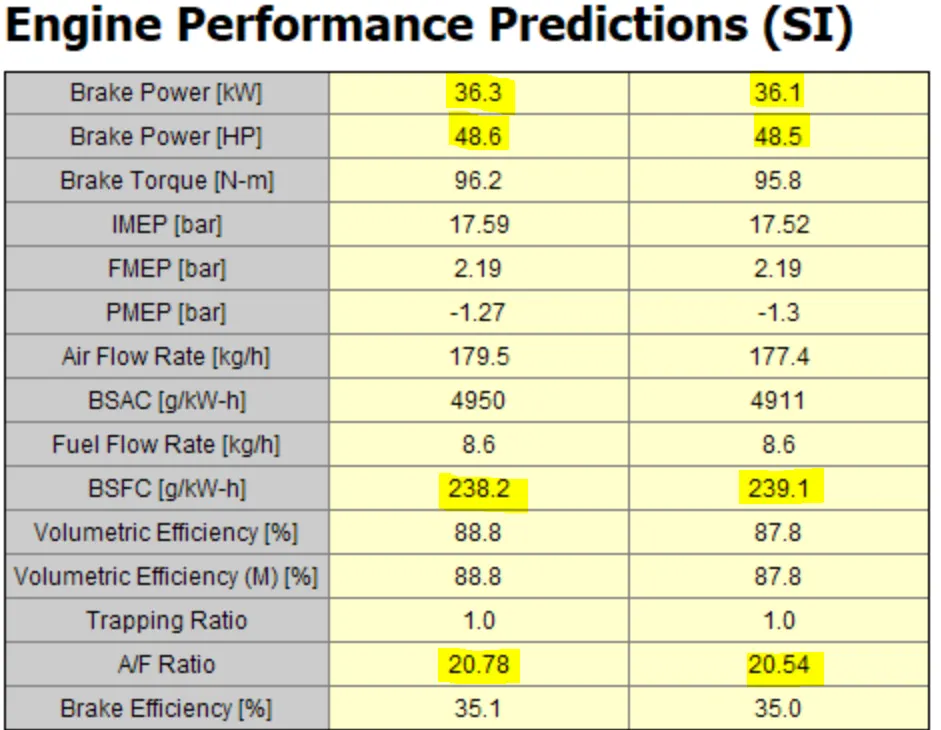
Plots comparision :

1.

2.

3. Time elapsed

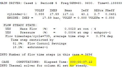
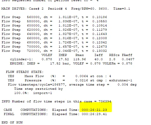
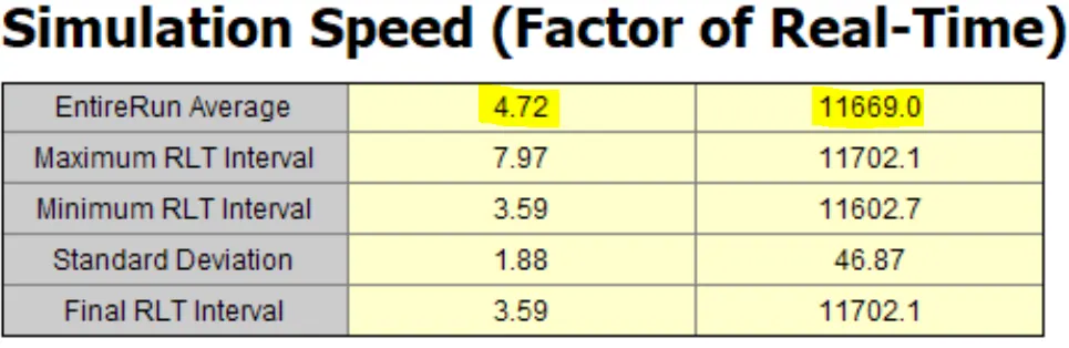
• We can clearly observe from above tables that there is variation in values i.e. error is found if discretizing length is more. This owes to inaccuruacy of solver assuming the flow and changes to be similar across varying lengths of intake pipe. Hence, discretizing is must when accuracy is required.
• Further, there is significant increase in time taken to perform simulation as discussed earlier ∆t ∝ ∆x, the discretized element length shouldn't be unnecessarily small as it increases the time step and shouldn't be of higher value to not capture the results accurately.

2. DISCRETIZATION OF INTAKE MANIFOLD

1. Import the STL file Plenum to GEM 3D to perform discretization.

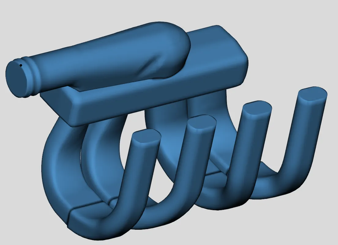
2. To divide into components we have to first discrete them using separate by curves method. Below is the image depicting dividing into different parts where there is abrupt changes in area.

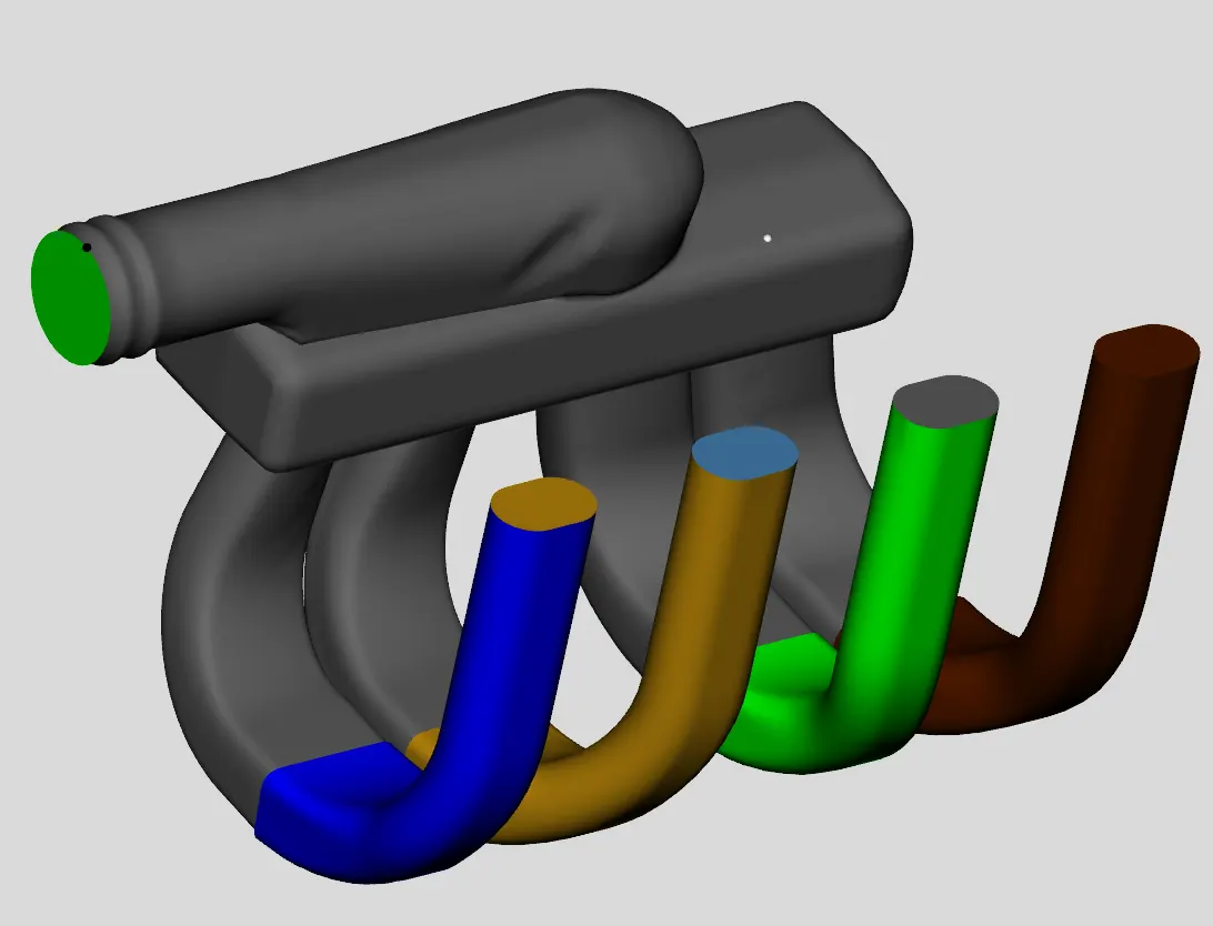
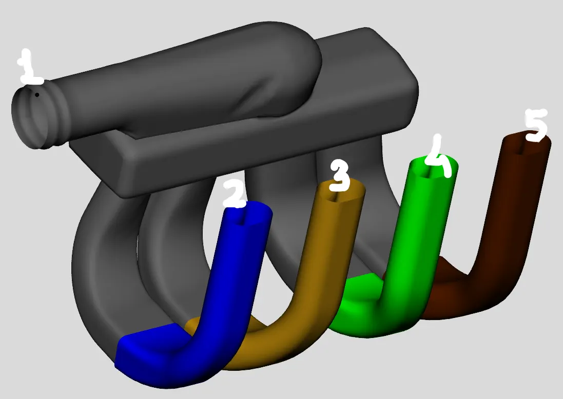
3. As the fluid enters and exits the pipe from intake and though the runners, openings are made then

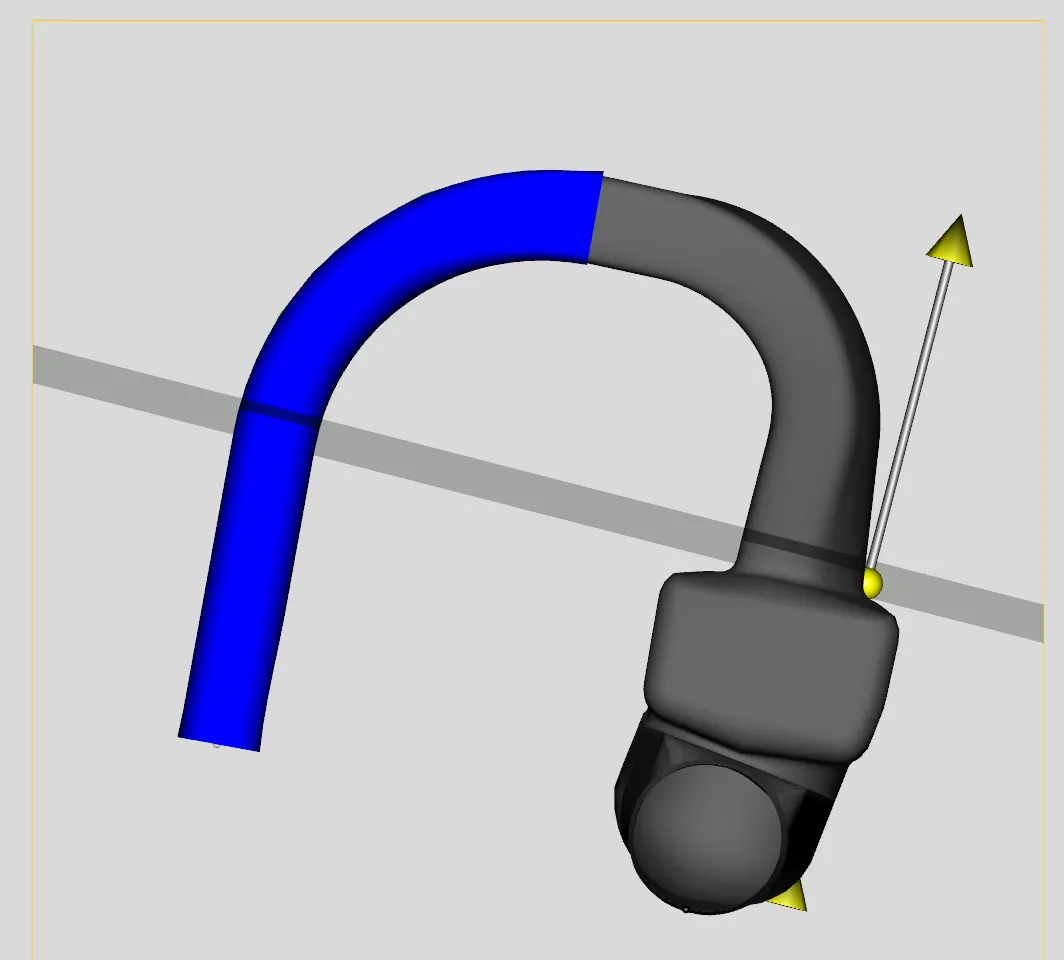
4. We proceed next to distinguish intake runners of runners from plenum from the outlet by using 3-points cuttting plane. Care must be taken that cutting plane ddoesn't cut off the plenum.

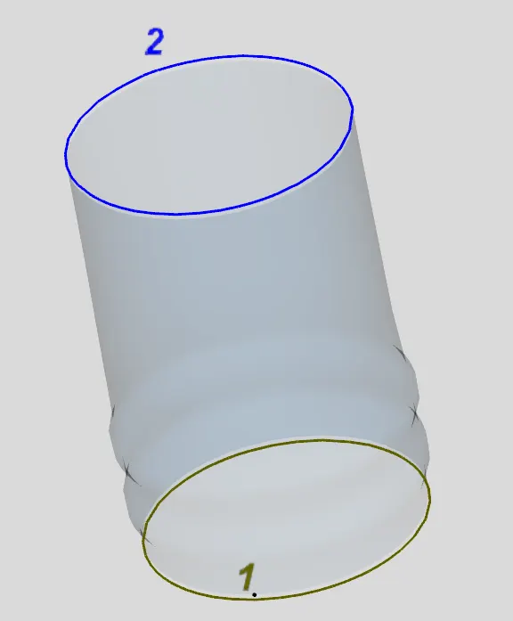
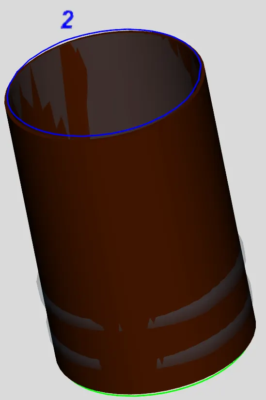
5. Now converting the intake-pipes(runner) into pipe of equal radius. i.e. Fig.1 to Fig. 2

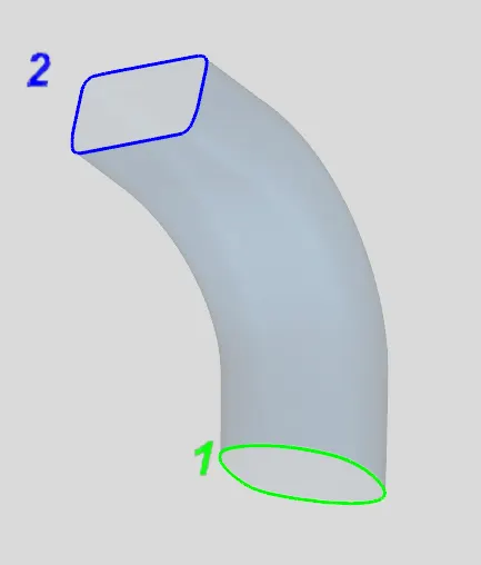
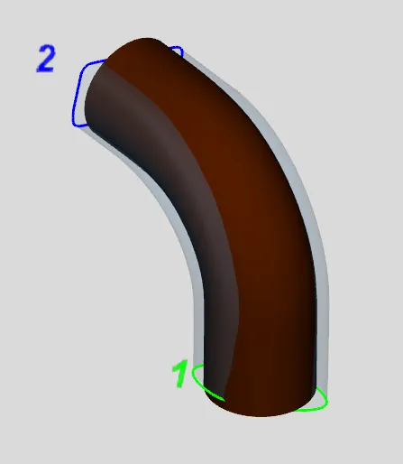
Fig. 1 Fig. 2

ii. Also converting for outlet runners

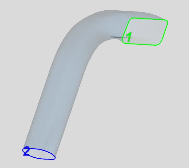
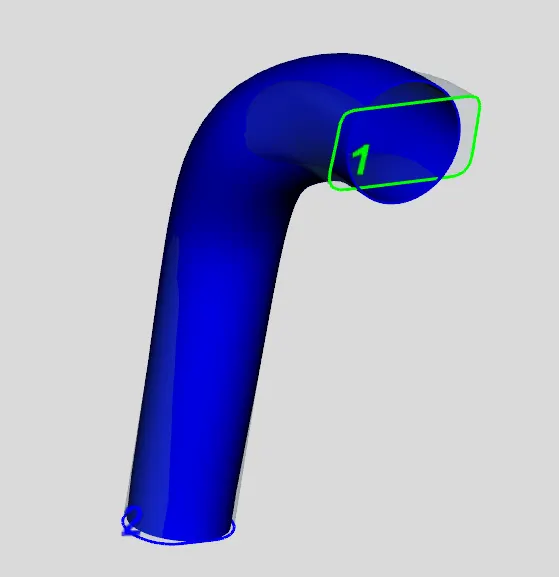
Fig. 1 Fig. 2

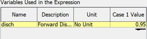
6. For better transitional flow from manifold to runner we need to add orifice connection manually using Add Connection with a forward discharge coefficient of 0.95.

ii. Further define the extension i.e. outlet from runners

7. Further, more cuts are performed near the intake-manifold to obtain a proper discretized model

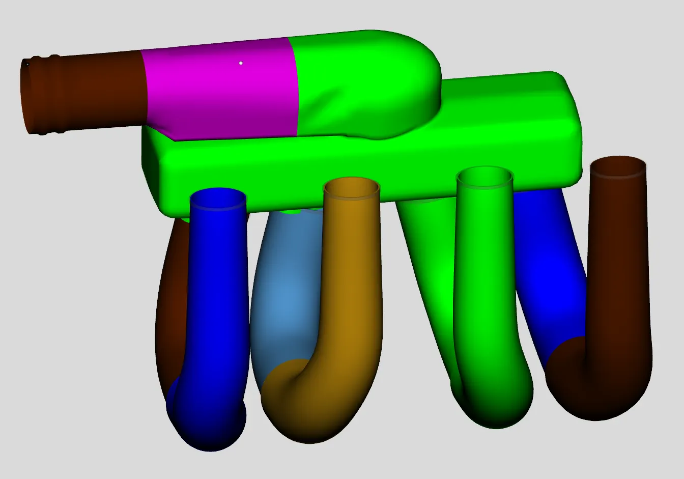
8. These shapes are converted into proper components and connections are added.

9. Then the pleunum is divided into components to easily identify the flow into runners.

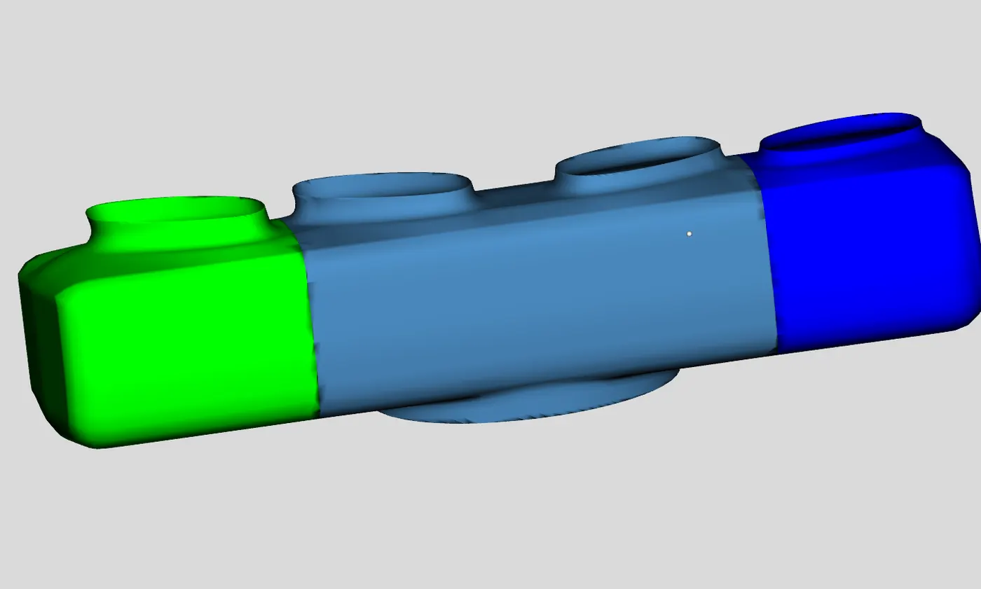
10. Using Flow connection tool gaps are repaired so as to avoid uninterrupted fluid flow. Upon the selection of tool it previews where they are to be repaired.

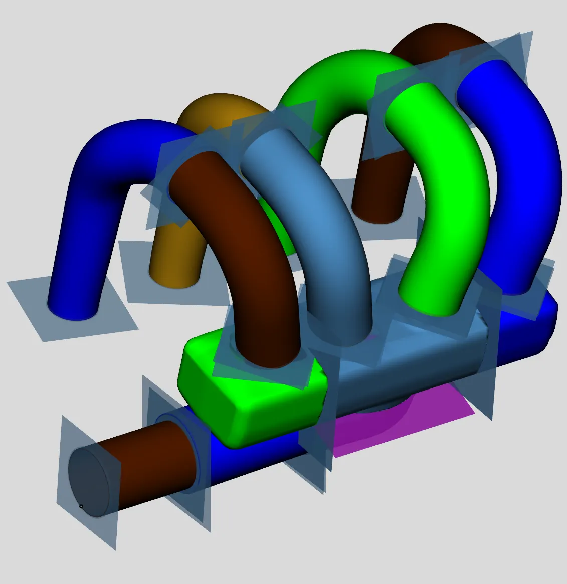
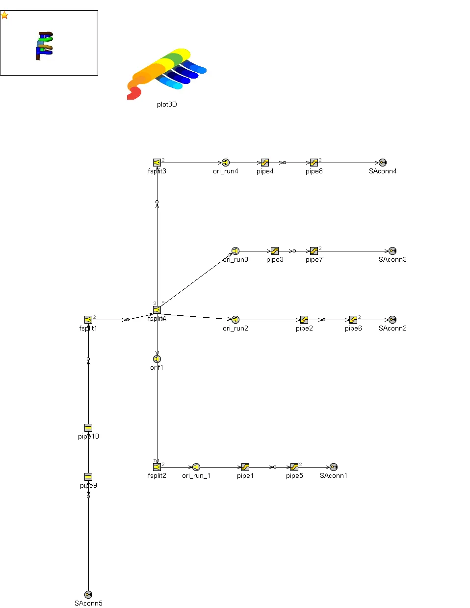
11. Using the export-GT model discretize it with custom setting as shown an open in GT-ISE model. After properly arranging the circuits we get the final connection.