ANIMATING THE MOTION OF A SIMPLE PENDULUM BY SOLVING SECOND ORDER DIFFERENTIAL EQUATION USING MATLAB AND OCTAVE
AIM :
To solve the second order Differential equation of a simple pendulum and animating its motion using MATLAB and OCTAVE.
The pendulum motion depends up on the newtons second law where it leads to forming the second order ODE.
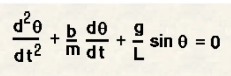
θ is the Angular displacement in radians.
b is damping factor in (kg/sec)
m is mass of the pendulum bob in Kg
g is acceleration due to gravity in (m/sec^2)
L is length of pendulum in m
Procedure :
The higher order ODE is broken into set of first order ODE's.
θ = θ1 ------> (1)
dθ/dt = dθ1/dt = θ2---------> (2)
substitute Equations 1 and 2 in the main equation
dθ1/dt = θ2
dθ2/dt = -(b/m)θ2-(g/L)sinθ1
Use of ode45 in MATLAB :
[tsol , ysol] = ode45(@(t,y)fname(t,y),[t0,tend],y0);
tsol , ysol = solution vectors . Matlab returns ysol value for each tsol value
fname = Function that returns dy =F(t,y)
t0 , y0 = Initial conditions representing y(t0)=y0
tend = Final value until which the solution is desired.
dy/dt = F(t ,y)
Code in matlab :
clear all
close all
clc
%damping factor in kg/sec
b=0.05;
%acceleration due to gravity in m/sec^2
g=9.81;
%length of pendulum in meters
l=1;
%mass of pendulum bob in kg
m=0.1;
%initial conditions for angular displacement(θ1) and angular velocity(θ2)
theta0=[0;5];
%time values
tspan=linspace(0,20,100);
%solving the second order ODE
[t,result]=ode45(@(t,theta) callfunc(t,theta,b,g,l,m),tspan,theta0);
%plotting
figure(1)
subplot(2,1,1)
p1=plot(t,result(:,1),'linewidth',2,'color','b')
xlabel('time')
ylabel('angular displacement')
hold on
subplot(2,1,2)
p2=plot(t,result(:,2),'linewidth',2,'color','r')
xlabel('time')
ylabel('angular velocity')
axis([0 10 -5 5])
legend([p1(1),p2(1)],'angular displacement','angular velocity')
theta=result(:,1);
ct=1;
%animation
for i=1:length(result)
    THETA=result(i,1)
    x0=0;
    y0=0;
    x1=l*sin(THETA);
    y1=-l*cos(THETA);
    figure(2)
    hold on
    plot([x0 x1],[y0 y1],'linewidth',4);
    plot(x1,y1,'-o','markersize',30,'markeredgecolor','g','markerfacecolor',[0.6 0 0]);
     plot(x0,y0,'-*','markersize',3,'markeredgecolor','g','markerfacecolor',[0.6 0 0]);
     axis([-2 2 -2 0])
     pause(0.005)
     M(ct)=getframe(gcf);
     ct=ct+1;
     clf()

end
movie(M)
videofile=VideoWriter('pendulumanimation.avi','uncompressed AVI')
open(videofile)
writeVideo(videofile,M)
close(videofile)
Function code :
function [dtheta_dt]=callfunc(t,theta,b,g,l,m)
theta1_dt=theta(1);
theta2_dt=theta(2);
dtheta1=theta2_dt;
dtheta2=(-(b/m)*theta2_dt)-((g/l)*sin(theta1_dt));
dtheta_dt=[dtheta1;dtheta2];
end
Code Explanation :
1) Taking the values of damping,length and mass of the pendulum bob
2) setting the initial conditions for displacement and velocity
3) Taking different time values using linspace command
4) Solving the second order DE of simple pendulum using ode45 command
5) The equations of single ODE is solved in seperate function and that function is called in the main program.
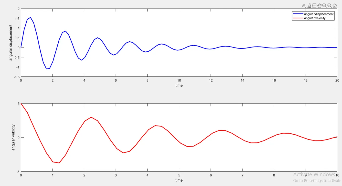
6) The first column of results indicates the angular displacement and the second column of results indicate angular velocity
7) plotting the curves for displacement and angular velocity by taking subplot command
8) The link and bob of the pendulum are created and the for loop is created for generating each and every position of the pendulum wrt to theta.
Animation :
getframe : It collects the frame and stores the frame in it
movie : It generates an animation using the frames collected
videofile=videoWriter() : It assigns file name and file format
open(videofile) : It opens the video file
writeVideo(videofile,M) : It writes the video with plot frames in array M
close(videofile) : It closes the video file
OUTPUT :
Animation link :
Octave code :
clear all
close all
clc
b=0.05;
g=9.81;
l=1;
m=0.1;
theta0=[0;5];
tspan=linspace(0,20,100);
[result]=lsode("callfunc",theta0,tspan);
figure(1)
subplot(2,1,1);
plot(tspan,result(:,1),'linewidth',2,'color','b');
subplot(2,1,2)
plot(tspan,result(:,2),'linewidth',2,'color','r');
ct=1;
THETA=result(:,1);
for i=1:length(result(:,1))
THETA1=THETA(i);
    x0=0;
    y0=0;
    x1=l*sin(THETA1);
    y1=-l*cos(THETA1);
    graphics_toolkit('gnuplot')
    figure(i+1)
    plot([-0.5 0.5],[0 0],'linewidth',4,'color','b');
    hold on
    line([x0 x1],[y0 y1],'linewidth',5,'color','g')
    hold on
    plot(x1,y1,'marker','o','markersize',20,'markerfacecolor','y');
    hold on
    grid on
     axis([-2 2 -2 1.5])
     graphics_toolkit('gnuplot')
     text=sprintf("pendulum%d.png",i)
     saveas(gca,text)
     end
Function code :
function [dtheta_dt]=callfunc(theta,t,b,g,l,m)
b=0.05;
g=9.81;
l=1;
m=0.1;
theta1_dt=theta(1);
theta2_dt=theta(2);
dtheta1=theta2_dt;
dtheta2=(-(b/m)*theta2_dt)-((g/l)*sin(theta1_dt));
dtheta_dt=[dtheta1;dtheta2];
end
Explanation :
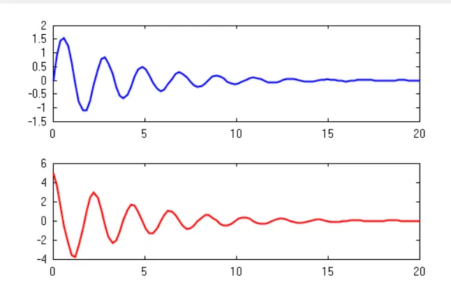
The entire code is similar to matlab except the animation and the ode45 command.In some octave versions ode45 doesnt support and in the place of ode 45 we have to use lsode command
Output :
Pendulum pics at different locations :
https://drive.google.com/drive/folders/1bihWSk_9nkjTnCAlSLHfupillhWrLPIL?usp=sharing
Animation in octave :
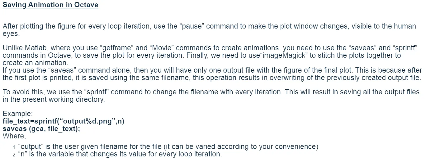
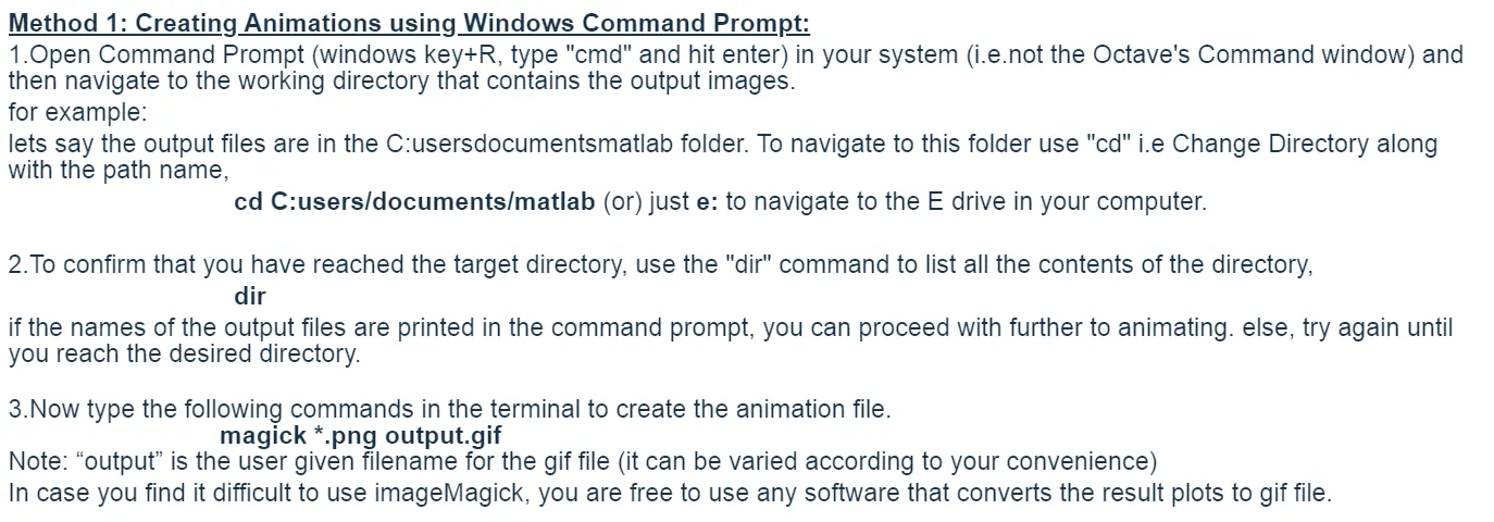
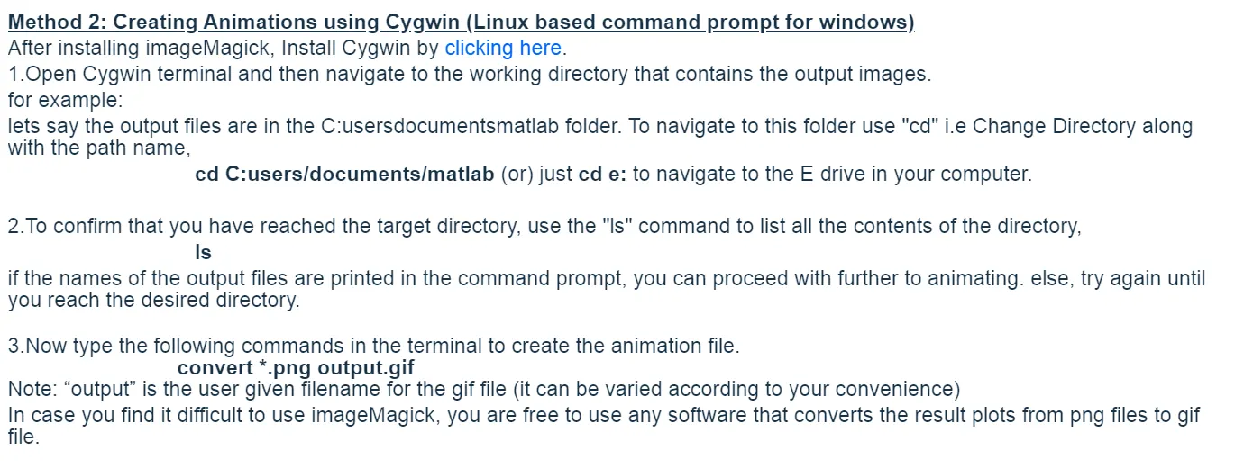
Image magic download :
https://imagemagick.org/script/download.php
Errors :
all errors are typos and can be rectified by error message displayed in command window