Air standard Cycle Programing in Matlab

ABOUT OTTO CYCLE

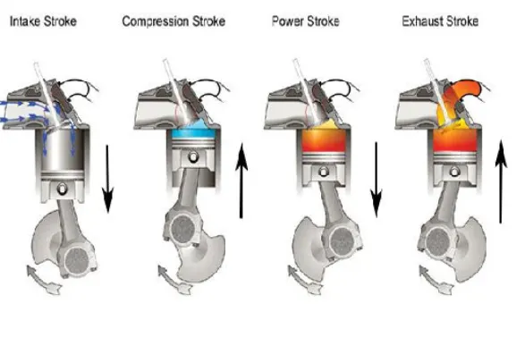
Otto Cycle is the theoretical thermodynamic cycle that describes the working of a spark-ignition engine. This type of spark-ignition engine is the most common type of engine used in automobiles.

The Otto cycle is the study of what happens to a mass of gas when it is subjected to changes in pressure, temperature, volume, adding heat, and removing heat. The system is the term given to the mass of gas that is subjected to these changes. Otto Cycle also studies the effect of this system on the environment. The effect in question here is the net output or the work generated by the Otto Cycle to move the automobile in which the engine is installed.

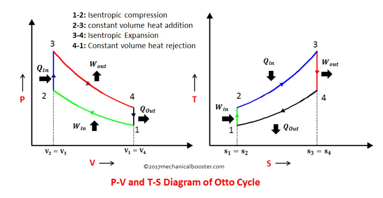
EXPLANATIONS AND FORMULAS USED IN PROGRAMMING

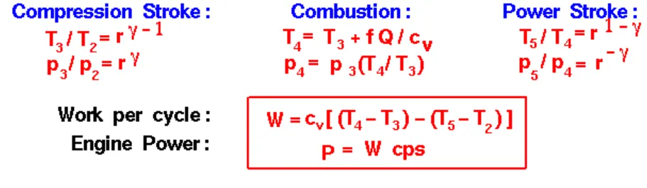
THERMAL EFFICIENCY = 1-(V2/V1)^gamma-1

FUNCTION PROGRAM FOR OTTO CYCLE

The following Program has been made to use as a function for the main program

function [v] =engine_kinematics(bore,stroke,con_rod,cr,start_crank,end_crank)


pr = stroke/2;
R = con_rod/pr;

v_s = pi/4*bore^2*stroke;
v_c = v_s/(cr-1);

theta = linspace(start_crank,end_crank,100)

%Using V/Vc=1+0.5(cr-1)[R+1-costheta-(R^2-sin^2theta)^0.5]

a=0.5*(cr-1)
b=R+1-cosd(theta);
c=(R^2-sind(theta).^2).^0.5;
v= (1+a*(b-c)).*v_c


end

To simplify the data entry process for the calculations of otto cycle this function is very helpful

Main Program

clear all
close all
clc

%Inputs
gamma=1.4
% State Variables

p1 = 101325
t1= 500
t3=2300

% Engine geometric parameters
bore=0.1
stroke=0.1
con_rod=0.15
cr=12

% Calculating Swept Volume and Clearance volume
v_swept = (pi/4)*bore^2*stroke
v_clearance = v_swept/(cr-1)

v1 = v_swept + v_clearance 
v2 = v_clearance

% State Variables at state point 2
%p2v2^gamma=p1v1gamma
%p2=p1*(v1/v2)^gamma=p1*cr^gamma
p2=p1*cr^gamma

%p1v1/t1=p2v2/t2 | t2=p2v2*t1/(p1v1)
t2=p2*v2*t1/(p1*v1)

constant_c=p1*v1^gamma;
v_compression=engine_kinematics(bore,stroke,con_rod,cr,180,0)
p_compression=constant_c./v_compression.^gamma

% State Variables at state point 3
v3=v2
%p3v3/t3=p2v2/t2 | p3=p2t3/t2
p3=p2*t3/t2

constant_c=p3*v3^gamma;
v_expansion=engine_kinematics(bore,stroke,con_rod,cr,0,180)
p_expansion=constant_c./v_expansion.^gamma

%State Variables at point 4
v4=v1
%p3v3^gamma=p4v4^gamma | p4=p3(v3/v4)^gamma

p4=p3*(v3/v4)^gamma

figure(1)
hold on
plot(v1,p1,'*','color','r')
plot(v_compression,p_compression)

plot(v2,p2,'*','color','r')
plot([v2 v2],[p2 p3])
% plot([v_compression,v_expansion],[p_compression,p_expansion],'color','b')
plot(v_expansion,p_expansion)
% plot([v_expansion,v_compression],[p_expansion,p_compression],'color','r')

plot(v3,p3,'*','color','r')
plot([v4 v4],[p4 p1])
plot(v4,p4,'*','color','r')
xlabel('Volume')
ylabel('Pressure')
legend('Isentropic Compression','Constant Volume Heat Add','Isentropic Exp','Constant Volume Heat Rej')

%Thermal Efficiency

thermal_eff=(1-(v2/v1)^(gamma-1))*100
Nth=thermal_eff

Result Plot

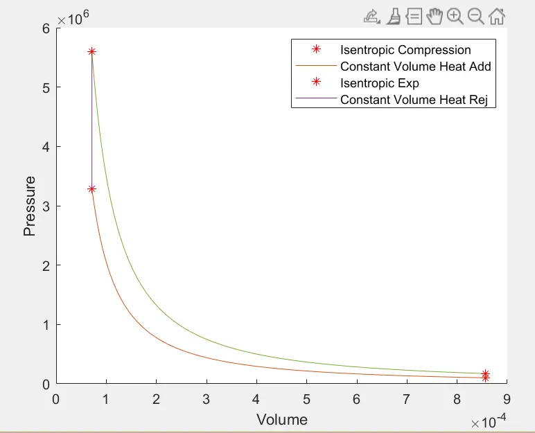
THERMAL EFFICIENCY

The Thermal Efficiency obtained is 62.98%