PV Diagram of an Otto Cycle

PV Diagram of an Otto Cycle

Aim: Creating a program in MATLAB to plot PV diagram of an Otto Cycle and calculate thermal efficiciency(`eta`).

Objective:

• Writing a program for Otto Cycle.
• Plotting a PV diagram.
• Determining the thermal efficiency of the engine.

Methodology:

Theory

Otto Cycle

An Otto Cycle is an idealized thermodynamic cycle that describes the functioning of a typical spark ignition piston engine. It is the thermodynamic cycle most commonly found in automobile engines.

The Otto cycle is a description of what happens to a mass of gas as it is subjected to changes of pressure, temperature, volume, addition of heat, and removal of heat. The mass of gas that is subjected to those changes is called the system. The system, in this case, is defined to be the fluid (gas) within the cylinder. By describing the changes that take place within the system, it will also describe in inverse, the system's effect on the environment. In the case of the Otto cycle, the effect will be to produce enough net work from the system so as to propel an automobile and its occupants in the environment.

The Otto cycle is constructed from:

• Top and bottom of the loop: a pair of quasi-parallel and isentropic process (frictionless, adiabtic reversible).
• Left and right sides of the loop: a pair of parallel isochoric process (constant volume).

The isentropic process of compression or expansion implies that there will be no inefficiency (loss of mechanical energy), and there be no transfer of heat into or out of the system during that process. The cylinder and piston are assumed to be impermeable to heat during that time. Work is performed on the system during the lower isentropic compression process.

Types of Engine that uses the Otto Cycle

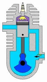
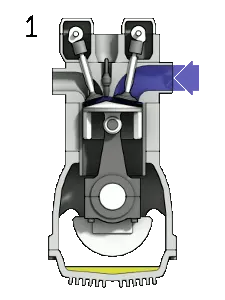
Fig: Two Stroke Engine Fig: Four Stroke Engine

Both of the engine is the spark ignited.

The Ideal Otto cycle

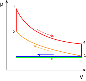
Figure 3. The PV diagram of an ideal Otto Cycle process. It consists of two isochoric, two adiabatic and two isobaric processes (for intake and exhaust)

The PV diagram (pressure-volume diagram) of the ideal Otto cycle is shown in Figure 3. This diagram models how the changes in pressure and volume of the working fluid (gasoline and air fuel) change due to the combustion of hydrocarbons which powers the movements of a piston, creating heat, to provide motion for a vehicle. There are expansion (increased volume chamber) piston motions—caused when the thermal energy is released from combustion—inducing work being done by the gas and on the piston. In contrast, when the piston does work on the gas, the engine chamber is being compressed (decreasing in volume).

It is important to note that Figure 3 depicts an ideal process for any engine using the Otto cycle. It describes the basic working steps in a gasoline engine. The slight modification which depicts a more realistic situation of the Otto Cycle's PV diagram for a two stroke and four stroke engine is explained on their respective pages. The work done by the engine can be calculated by solving the area of the closed cycle.

The following describes what occurs during each step on the PV diagram, in which the combustion of the working fluid—gasoline and air (oxygen), changes the motion in the piston:

Green line: Referred to as the intake phase, the piston is drawn down to the bottom to allow the volume in the chamber to increase so it can "intake" a fuel-air mixture. In terms of thermodynamics, this is referred to as an isobaric process.

Process 1 to 2: During this phase the piston will be drawn up, so it can compress the fuel-air mixture that entered the chamber. The compression causes the mixture to increase slightly in pressure and temperature—however, no heat is exchanged. In terms of thermodynamics, this is referred to as an adiabatic process. When the cycle reaches point 2, that is when the fuel is met by the spark plug to be ignited.

Process 2 to 3: This is where combustion occurs due to the ignition of fuel by the spark plug. The combustion of the gas is complete at point 3, which results in a highly pressurized chamber that has a lot of heat (thermal energy). In terms of thermodynamics, this is referred to as an isochoric process.

Process 3 to 4: The thermal energy in the chamber as a result of combustion is used to do work on the piston—which pushes the piston down—increasing the volume of the chamber. This is also known as the power stoke because it is when the thermal energy is turned into motion to power the machine or vehicle.

Purple line (Process 4 to 1 and exhaust phase): From process 4 to 1, all waste heat is expelled from the engine chamber. As the heat leaves the gas, the molecules lose kinetic energy causing the decrease in pressure. Then the exhaust phase occurs when the remaining mixture in the chamber is compressed by the piston to be "exhausted" out, without changing the pressure.

Under the cold air-standard assumption, the thermal efficiency of the ideal Otto cycle is

Process 1-2 and process 3-4 are isentropic. Thus,

Since v₂ = v₃ and v₄ = v₁,

Considering all the relations above, the thermal efficiency becomes,

where r is the compression ratio and k is the specific heat ratio.

The expression of thermal efficiency under cold air-standard assumption is only a function of the compression ratio. Thus, a higher r can generate a higher thermal efficiency. But when higher r is used, the temperature of the air-fuel mixture may rise above the auto ignition temperature of the fuel during the compression process, and will cause an early and rapid burn before the spark ignition. This early and rapid burn produces an audible noise, which is called engine knock. Engine knock in spark-ignition engine cannot be tolerated since it hurts performance and can cause engine damage. Thus there is an upper limit of compression ratio for spark-ignition engines.

Fig: Relation between Thermal Efficiency and Compression Ratio with k =1.4

Program to find thermal efficiency and create PV diagram

Program for an Otto Cycle

To begin writing the program, we first need to have the initial input that we will use to find the Otto Cycle. The following are the values we will use it for our programming.

`gamma`=1.4

`pressure` = 101325 N/m²

T1 = 500 K

T3 = 2300 K

The above are the initial condition we have used as an input.

%A program to find PV diagram of an Otto Cycle
clear all
close all
clc

%Input
gamma=1.4;                       %Dimensionless

%State Variation
p1 = 101325;                     %N/m^2       
t1 = 500;                        %K
t3=2300;                         %K

%Engine generic parameter
bore = 0.1;                      %m^2
stroke = 0.1;                    %m
con_rod = 0.2;                   %m
cr = 12.5;                       %Dimensionless

%Calculating the swept volume and swept clearance
v_swept = (pi/4)*bore*2*stroke;
v_clearance = v_swept/(cr-1);
v1 = v_swept+v_clearance;
v2=v_clearance;

%State variables at state point 2
p2=p1*cr^gamma;
constant_c=p1*v1^gamma;
V_compression= piston_kinematic(bore,stroke,con_rod,cr,180,0);
P_compression = constant_c./V_compression.^gamma;
t2=p2*v2*t1/(p1*v1);

%State variables at state point 3
v3 = v2;
p3=p2*t3/t2;
constant_c=p3*v3^gamma;
V_expansion= piston_kinematic(bore,stroke,con_rod,cr,0,180);
P_expansion = constant_c./V_expansion.^gamma;

%State variables at state point 4
v4=v1;
p4=p3*(v3/v4)^gamma;

%Plotting
figure(1)
hold on
title('PV Diagram (Otto Cycle)')
xlabel('Volume(m^3)')
ylabel('Pressure(N/m^2)')
plot(v1,p1,'*','color','r');
plot(V_compression,P_compression,'-.','color','r');
plot(v2,p2,'*','color','r');
plot(v3,p3,'*','color','r');
plot(V_expansion,P_expansion,'-.','color','r');
plot(v4,p4,'*','color','r');
plot([v1,v4],[p1,p4],'-.','color','r');
plot([v3,v2],[p3,p2],'-.','color','r');

%Thermal Efficiency
Efficiency = 100*(1-(1/cr^(gamma-1)));
sprintf('The thermal efficiency is = %.2f percent',Efficiency)

At, first we begin our program, that will clear all the previous values stored in result window, and clear everything from command window.

We, put the initial value of `gamma`in gamma variable as 1.4. The remaining value that we input are bore diameter in bore variable as 0.1 m² , stroke length in stroke variable as 0.1 m, connecting rod length in con_rod variable as 0.2 m and compression ratio in cr variable as 12.5. We will also input pressure in p1 variable as 101325 N/m², temperature at point 1 as t1 and point 3 as t3 is taken as 500 K and 2300 K, respectively.

We then input the formula to calculate 'Swept Volume' and 'Clearance Volume'. We will store their values in v_swept and v_clearance. We then give the other relation and input their values in every state using the above equations for Otto Cycle. This way we write equations to find pressure, temperature and volume at every point of the cycle.

We will also put thermal efficiency equation to calculate efficiency of the Otto Cycle, and input this result in variable 'Efficiency'.

Lets assume, in the programming we do not mention function and call it back, and the coding for plotting we used is:

figure(1)
hold on
plot(v1,p1,'*','color','r');
plot(v2,p2,'*','color','r');
plot(v3,p3,'*','color','r');
plot(v4,p4,'*','color','r');
plot([v1 v2 v3 v4 v1],[p1 p2 p3 p4 p1],'color','b');

If, we had proceeded with the coding mentioned below plotting result, we would have got the result as;

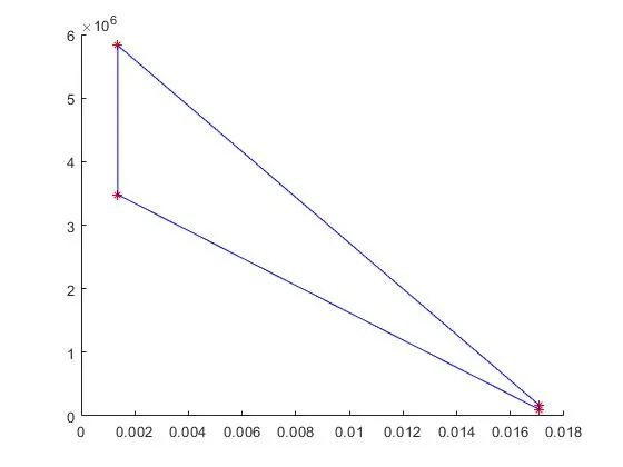
Fig: Incorrect depiction of PV diagram

The reason being that, the process is isentropic and not linear and the output we have got is incorrect. Not that it is wrong for constant volume process, but wrong for compression and expansion process.

As a result, we will use a function and call it for every changing position of Pressure and Volume during compression and expansion.

In another code as below, we have craeted the function called as 'piston_kinematic' with variable that will be given by user are bore, strokem con_rod, cr, start_crank and end_crank. The crank pin radius is denoted as 'a'. Crank pin radius is half of stroke length. Ratio of connecting rod length is denoted 'R', which is equal to connecting rod length divide by crank pin radius. Here too, we will give the equation to calculate swept volume and clearance volume at varying degree of theta.

Function for an Engine Kinematics

%Function to be recalled for Piston Kinematic of Otto Cycle
function [V] = piston_kinematic(bore,stroke,con_rod,cr,start_crank,end_crank)

%Generic function
a = stroke/2;
R = con_rod/a;

%Calculating the swept volume and swept clearance
v_s=(pi/4)*bore*2*stroke;
v_c=v_s/(cr-1);

%Angle of piston
theta=linspace(start_crank,end_crank,100);

%Isentropic geometric Relationship
term1=0.5*(cr-1);
term2=R+1-cosd(theta);
term3=(R^2-sind(theta).^2).^0.5;

V=(1+term1*(term2-term3))*v_c;
end

Using linspace function we will split the input value of theta in 100 values, and store tjose value in an array form in a variable called theta.

The ratio of Volume to Clearance volume is denoted as V, and is given by the following equation;

`frac{V}{Vc}`= 1 + `frac{1}{2}`(Rc - 1)[R + 1 -cos`theta` - (R^2 - sin^2 `theta`)^`frac{1}{2}`]

This is a pretty big equation to write in a MATLAB, so we will split this into small portion and assign it into different variables.

They are as follow:

term1 = `frac{1}{2}`(Rc - 1)

term2 = R + 1 -cos`theta`

term3 = (R^2 - sin^2 `theta`)^`frac{1}{2}`

The final equation will be very simple to make equation as. As we are calculating Volume, we will multiply clearance volume to the right.

Coming back to actual code;

Here, we will call back piston_kinematic function to calculate Compression Volume(V_compression).

The equation of constant using pressure and volume is given as;

Constant = P x V^`gamma`

So using constant_c varaiable we will find pressure during compression(P_compression).

The same will be done to calculate Expansion Volume(V_expansion).

Using the same constant equation we will find pressure during expansion(P_expansion).

The only difference will be, for finding Compression Volume we will using start crank angle as 180 degree and end crank angle as 0 degree and during Expansion of Volume we will using start crank angle as 0 degree and end crank angle as 180 degree.

This function is called back in the first code.

While plotting, using just p1,p2,p3,p4 and v1,v2,v3,v4 we will plot pressure and volume point of cycles.

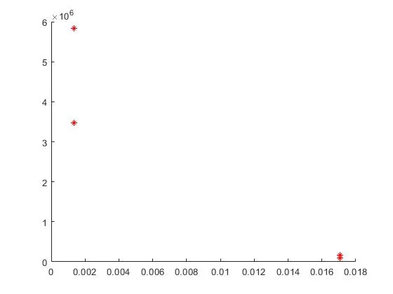
Fig: Different Pressure v/s Volume point at cycle

Using P_compression, V_compression and P_expansion, V_expansion, we will plot the curve using dash dot point. As, the cycle between point 2,3 and 4,1 is constant volume, we will simply denote it by straight line. We will plot straight line using dash doing line between 2,3 and 4,1.

Lets assume, we had a code which had input variables directly, like below;

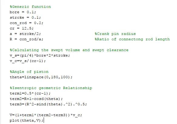
Using this code, if we were to find the the plot for theta against V for theta values between 0 and 180, the graph would have looked like;

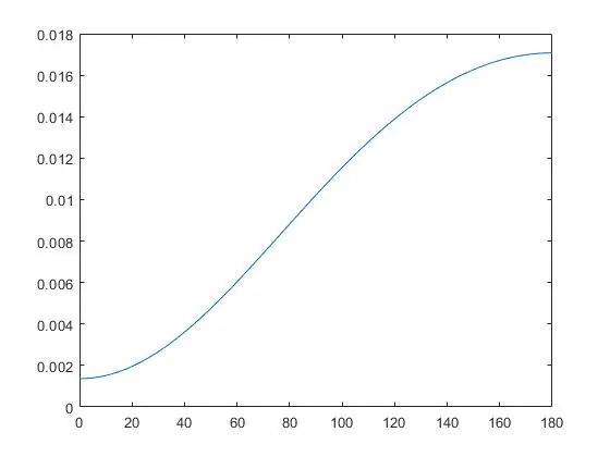
Fig: Proof that volume expansion and compression process is not linear

The above graph is further proof that the Volume compression and expansion cycle process does not have a linear relationship with Pressure during compression and expansion cycle, respectively.

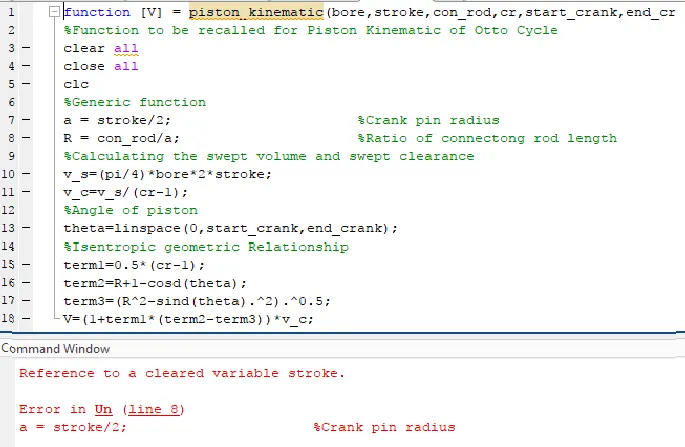
In above code, we did define the function, but the reason it did not execute is because we did not close the function using 'end'. By closing the function with 'end' we can close the function command.

Result:

The Pressure Volume diagram for an Otto Cycle, with the initial input mentioned above is as follow;

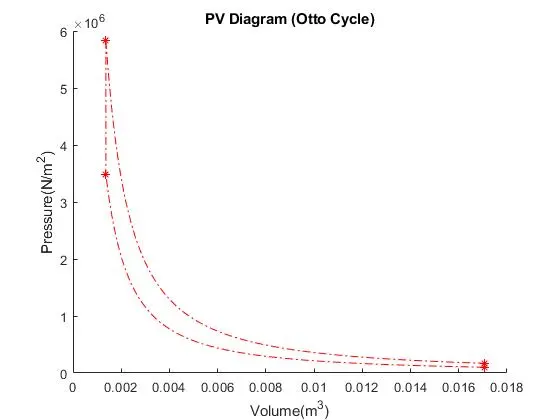
Fig: Actual PV diagram of an Otto Cycle

The thermal efficiency (`eta`) = 63.59 %

Fig: Thermal Efficiency

Learning Outcome:

• Learned the basic of Otto Cycle
• Understood the function command in application of 'Air Standard Cycle'.
• Learned plotting of graph for problems where the curves are not linear.

Conclusion:

Created a program to plot PV diagram of an Otto Cycle as well as calculated the thermal efficiency(`eta`).