Air Standard Cycle

Calculation of thermal efficiency and plotting of PV diagram of an OTTO CYCLE using MATLAB.

Theory:

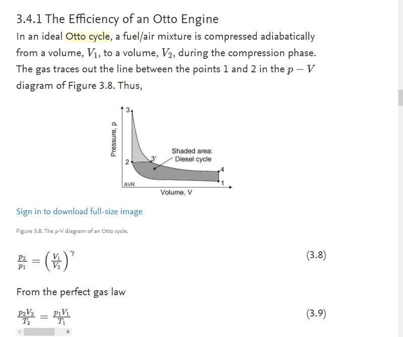
Otto cycle is an idealized thermodynamic cycle that describes the functioning of a typical spark ignition piston engine.

The processes are described by:

• Process 1–2 is an adiabatic compression of the charge as the piston moves from bottom dead center to top dead center.
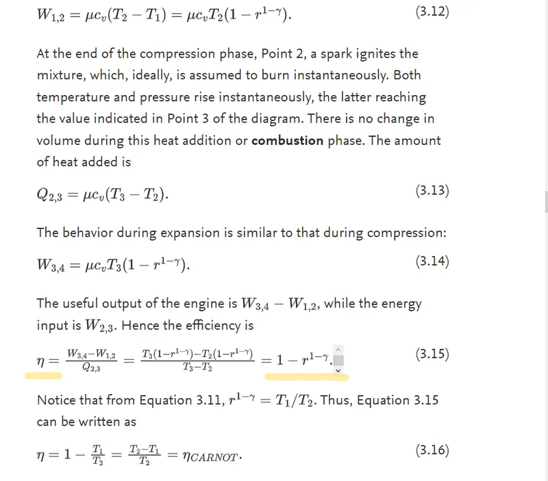
• Process 2–3 is a constant-volume heat transfer to the working gas from an external source while the piston is at top dead center. This process is intended to represent the ignition of the fuel-air mixture and the subsequent rapid burning.
• Process 3–4 is an adiabatic expansion (power stroke)
• Process 4–1 completes the cycle by a constant-volume process in which heat is rejected from the air while the piston is at bottom dead center.

%state variables
p1 = 101325;
t3 = 500;

%inputs
gamma = 1.4;
t3 = 2300;

%engine geometric parameters
bore = 0.1;
stroke = 0.1;
con_rod = 0.15;
cr = 12;

%calculation of swept volume and clearance volume
v_swept = (pi/4)*bore^2*stroke;
v_clearance = v_swept/(cr-1);


v1 = v_swept + v_clearance;
v2 = v_clearance;

%state variables at state point 2

%p2v2^gamma = p1v1^gamma
%p2 = p1(v1/v2)^gamma = p1(c_r)^gamma

%compression ration is equal to v1 divided by v2;

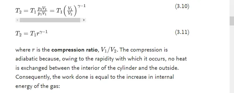
p2 = p1 * cr^gamma;


%from the perfect gas law, we can calculate temperature at state point 2
%p1v1/t1 =p2v2/t2 | t2 =p2v2t1 /p1v1

t2 = p2*v2*t1/(p1*v1);

%calculation of compression volume and pressure,which is from state point 1 to state point 2
constant_c = p1*v1^gamma;
V_compression = engine_kinematics(bore,stroke,con_rod,cr,180,0)
P_compression = constant_c./V_compression.^gamma;


%state variables at state point 3
v3 = v2;

%p3*v3/t3=p2*v2/t2 | p3 = p2*t3/t2;
p3 = p2*t3/t2;

%similarly here we calculated expansion volume and pressure, which go from point 3 to point 4
constant_c = p3*v3^gamma;
V_expansion = engine_kinematics(bore,stroke,con_rod,cr,0,180);
P_expansion = constant_c./V_expansion.^gamma;

%state variables at state point 4
v4 = v1;

%p3v3^gamma = p4v4^gamma| p4 = p3(v3/v4)^gamma
p4 = p3*(v3/v4)^gamma;

%plotting

figure(1)
hold on
plot(v1,p1,'*','color',r)
plot(V_compression,P_compression) %in order to draw a line from point 1 to point 2
plot(v2,p2,'*','color','r')
plot(v3,p3,'*','color','r')
plot(V_expansion,P_expansion) %in order to draw a line from point 3 to point 4
plot(v4,p4,'*','color','r')

%to draw a line of isochoric heat addition from point 2 to point 3,I did following plotting
plot([v2 v3],[p2 p3])

%calculation of thermal_efficiency
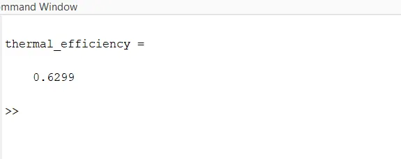
thermal_efficiency = 1 - (1/(cr)^(gamma-1))

Engine kinematics function,which was called inside the below code in calculation of compresion and expansion volumes and pressures.d

function [V] = engine_kinematics(bore,stroke,con_rod,cr,start_crank,end_crank)

Ena = stroke/2;
R = con_rod/a;

v_swept = (pi/4)*bore^2*stroke;
v_clearance = v_swept/(cr-1);

theta = linspace(start_crank,end_crank,100);

term1=0.5*(cr-1);
term2=R+1-cosd(theta);
term3=(R^2-sind(theta).^2).^0.5;

V = (1+term1*(term2-term3)).*v_clearance;

end

The result of thermal efficiency:

PV-Diagram of an Otto cycle:

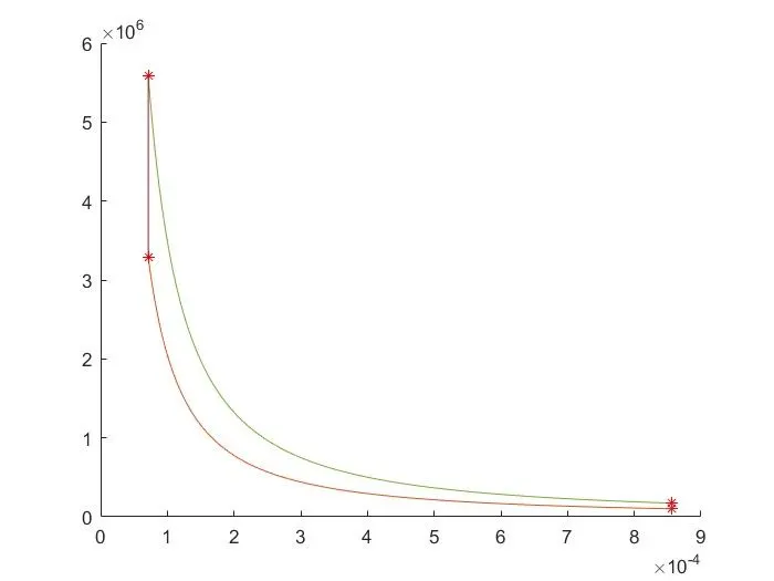
SUMMARY:

Otto cylcle was studied in this project, using matlab pv-diagram of otto cycle and also its thermal efficiency were figured and obtained.