Ahmed Body Challenge

Objective

• To study the importance of ahmed body model and the significance effect of the point of separation and the reason for the negative pressure in the wake region.
• To run the steady state simulation of the flow over the ahmad body.
• To plot the velocity and pressure contours. Also plot the vectot plot which clearly shows the wake region. And also display the graphs of the lift and drag coefficients.
• Perform the grid independency test and provide the values of drag and lift with each case.

As the burning of fossil fuels becomes a more pressing issue, manufacturers are introducing more fuel efficient cars to the market. One main contributor to fuel burn is the car’s aerodynamic drag. Complexly shaped, cars are very challenging to model and it’s difficult to quantify the aerodynamic drag computationally. The Ahmed body is a benchmark model widely used in the automotive industry for validating simulation tools. The Ahmed body shape is simple enough to model, while maintaining car-like geometry features.

The drag coefficient quantifies the resistance of an object in a fluid environment. It is not an absolute constant for a body’s shape because it varies with the speed and direction of flow, object shape and size, and the density and viscosity of the fluid. The lower the drag coefficient of an object, the less aerodynamic or hydrodynamic drag occurs. In terms of a car, the lower the drag coefficient, the more efficient the car is. As well as affecting the top speed of a vehicle, the drag coefficient also affects the handling. Cars with a low drag coefficient are sought after, but decreasing the drag drastically can reduce the downforce and lead to loss in road traction and a higher chance of car accidents.

Most cars have an average drag coefficient of between 0.30 and 0.35. Boxy cars have a higher number, like the HUMMER® H2 vehicle at .57, while more streamlined and agile cars have a lower number, like the Mercedes-Benz® C-Class® vehicle at 0.24. Again, this is just an average measurement. The exact drag coefficient of a car varies with the Reynolds number and various other factors.

There are certain ways to modify a car to optimize its aerodynamics and decrease the drag coefficient. To streamline the exterior, you can remove certain aftermarket items such as the roof rack, mud flaps, spoilers, and radio antenna. Professional car racers also take off their windshield wipers and side mirrors, but this isn’t recommended for the average driver! You can also add wheel covers, a partial grille block, an under tray, fender skirts, and a modified front bumper to improve the drag coefficient and make your car stand out in the process.

What Is an Ahmed Body?

The Ahmed Body was first created by S.R. Ahmed in his research “Some Salient Features of the Time-Averaged Ground Vehicle Wake” in 1984. Since then, it has become a benchmark for aerodynamic simulation tools. The simple geometrical shape has a length of 1.044 meters, height of 0.288 meters, and a width of 0.389 meters. It also has 0.5-meter cylindrical legs attached to the bottom of the body and the rear surface has a slant that falls off at 40 degrees.

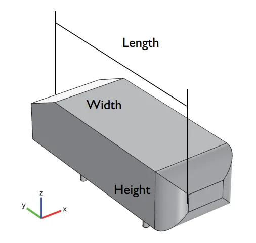
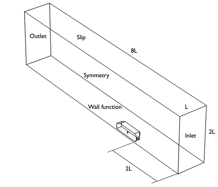
Dimensions of Ahmad body geometry

Steps to be performed to prepare geometry for meshing

• In the first step we import the geometry and set the dimensions into meters.

• In the second step, we create the enclosure. For the ahmad body we run the simulation in a closed environment. For this it is required for the solver to extract the volume data within defined boundary condition.

• Now we adjust the length and height of the enclosure body.

• Next we adjust the width parameter of of the enclosure body

• After adjusting all the parameters we click on the right mark then the enclosure is created.

• Hit Esc to exit the enclosure tool. Next go to design in the tool bar and click on plane to generate the plane and then click on the origin, then we saw the three plane. One plane is perpendicular to x-axis and other is perpendicular to y-axis and third is perpendicular to z-axis.

• Then hit Esc to exit the plane mode. Then select the plane 1 and click on the section mode. And we see the ahmad body is automatically cut in. Then hit Esc to exit the tool.

• To capture the wake region properly we create another enclosure, whose dimensions are given below.

• 3D view of the double enclosure is

• To reduce the computational effort we are taking the half geometry by using the spilt tool. For this first of all enable the plane1, then go to design and click on the spilt body tool and click on the front body and then click on the selected plane and by using cutter cut the front part of the enclosure geometry. Repeat the same process by spilting the inner enclosure.

• Then go to section mode. In the tool bar go to the prepare and then click on the interface it automatically eliminate the overlapping of hatch pattern.Next step we share the topology of the inner box with outer box. For this in the tool bar go to workbench and click on share and click on right mark.

• Click on the ahmad body and in the peoperties choose the share topology option.
• delete the plane and then right click in the enclosure 1 and enclosure 2 and move into the new component and name it ahmad body.
• close the space claim.

Mathematically Models

Governing equations

For all types of flows Ansys fluent solves the conservation equations for mass and momentum.

The equation for the mass, momentum can be written as the follows

`frac{partialrho}{partialt}+nabla.(rho barv)=S_m` (1.1)

equation (1.1) is the general form of the mass conservation equation and is valid for incompressible and as well as compressible flows. The source `S_m`is the mass added to the continuous from the dispersed phase.

`frac{partial}{partialt}(rhobarv)+nabla.(rhobarv barv)=-nablap+nabla.(tau)+rhobarg+barF` (1.2)

Where p is the static pressure , `tau`ia the stress tensor, `rho bar g`and `barF`are the gravitional body forces and extrenal body force.

In this model we used the k-omega SST model, whose description are given below

The shear stress transport (SST) k-omega model was developed by Menter to effectively blend the ronust and accurate formulation of the k-omega in the near-wall region with the freestream independence of the k-epsilon model in the far field. To achieve this, the k-epsilon model is converted into k-omega formulation. The SST k-omega is similar to the standard k-omega model,but includes the following refinements:

• The standard k-omega model and the transformed k-epsilon mpodel are both multiplied by a blending function and both models are added together. The blending function is designed to be one in the near wall region, which activates the standard k-omega model, and zero away from the surface, which activate the transformed k-epsilon model.
• The SST model incorporates a damped cross-diffusion derivatives term in the omega equation.
• The definition of the turbulent viscosity is modified to account for the transport of the turbulent shear stress.
• The modeling constants are different.

These feature makes the k-omega model more accurate and reliable for a wider class of flows.(for example adverse pressure gradients flows, airfoils, transonic shock waves) than the standard k-omega model.

`frac{partial}{partialt}(rhok)+frac{partial}{partialx_i}(rhoku_i)=frac{partial}{partialx_j}(rhoku_j)+frac{partial}{partialx_j}(Gamma_kfrac{partialk}{partialx_j})+G_k-Y_k+S_k`

`frac{partial}{partialt}(rhoomega)+frac{partial}{partialx_j}(rhoomegau_j)=frac{partial}{partialx_j}(rhoomegau_i)+frac{partial}{partialx_j}(Gamma_omegafrac{partialomega}{partialx_j})+G_omega-Y_omega+S_omega`

In the above equation `G_k`represents the production of kinetic energy and `G_omega` is the production of omega.`Gamma_k` and `Gamma_omega` represents the effective diffusivity of k and omega. `Y_k` and `Y_omega` represents the dissipation due to turbulence. `D_omega` represents the diffusion term. `S_k`and `S_omega`are user defined source term.

Meshing

Case Number	Outer Enclosure	Inner Enclosure	Ahmad body	Wheels	Bottom	Total number of cells
Case-1	Method: Multizone Element size: 6e-02 m Maximum element size:6e-02 m	Body sizing Element size:2.7e-02 m	Boundary layer Method: Named Selection Boundary: Car_wall Inflation layers: 11 Growth Rate: 1.2 Maximum thickness: 8e-04 m	Edge sizing No of divisions: 20	Inflation option: Total thickness Inflation layers: 6 Growth Rate: 1.15 Maximum thickness: 1e-03 m	Nodes:135961 Elements:458626

Meshing procedure:

• In the first step we set the mesh settings for the outer enclosure. We used the multizone method for the outer enclosure region. we used the 0.06 m size for the element size and maximum element size for the elements is also gave 0.06 m so that we will get a perfect looking mesh for the outer enclosure as shown below.

• Body sizing has been given for the inner enclosure with element size 0.0027.
• We are more interested in capturing the physics of flow near the ahmad body. To capture this with more accuracy we need more cells and nodes. That's why we reduce the size of element as we approach towards the ahmad body from the outer enclosure.
• Six inflation layers have been provided for the ahmad body(car_wall) with maximum layer thickness as 8e-04 m with growth rate 1.2. The calculation of maximum layer thickness based on the target Y+ will be explained in the below. but here i also do some hit and trial in maximum layer thickness to got the accurate results.
• six onflation layers have been provided with maximum thickness 1e-03 m with growth rate 1.15 in the bottom wall. This has been given to capture the physics of the flow more accurately as we also gave the wall boundary condition to this face.
• Edge has been given to the wheels with 20 no of divisions. This has been given to retain the cylindrical/circular shape, otherwise it might be disturbed and reduce the accuracy of the results.

In the following image we see the more finer case mesh. This is the 2D view of the mesh for batter visualization.

Calculation of first layer thickness using Y+ values

In the turbulent boundary layer region flow near the wall has been analyzed in terms of three layers.

• The inner layer, or sublayer, where viscous shear dominates
• The outer layer, or defect layer, where large scale turbulent eddy shear dominates
• The overlap layer, or log layer, where velocity profiles exhibit a logarithmic variation

The existence of all these layers in the boundary layers made the near-wall treatment nonlinear and inconsistent. The early researcher found it very difficult to find the numerical trend line which matches the experimental results. Many found that there is some relationship between velocity and wall distance, but fitting that in some equation was not easy for them. Finally, In 1905, Prandtl and his student nikuradse normalized the axes into y+(the axis that is used to be the distance) and u+(the axis that is used to be velocity). They also wrote an equation that would fit u+ and y+ near the wall.

if we intend to resolve the effects near the wall i.e., in the viscous sublayer then the size of the mesh size should be small and dense enough near the wall so that almost all the effects are captured. But in some cases, if the wall effects are negligible then there is an option of including semi-empirical formulae to bridge between the viscosity affected region and fully turbulent region, and in this case, the mesh need not be dense or small near the wall i.e., the coarse mesh would work. Near-wall modeling it is well-known that the mesh size should be small enough, however then the question follows is how small? Thus, here comes the concept of y+, and based on the y+ value the first cell height can be calculated. The near-wall region is meshed using the calculated first cell height value with gradual growth in the mesh so that the effects are captured and avoiding overall heavy mesh count.

During the meshing for a suitable size for first the layer of the grid cells (inflation layer) so that `Y^+`is in the desire range.

we require the following inpits for the calculation of first layer thickness

free stream velocity = 25m/s, Density = 1.225 `frac{kg}{m^3}`, Dynamic Viscosity = 1.7894e-05`frac{kg}{ms}`, Length = 1.044[m],

Reynold number=`frac{rhovD}{mu}`= `frac{(1.225)(25)(1.004)}{1.7894e-05}=1.8e06.`

Friction coefficient = 0.058 `Re^(-0.2)` , For external flows

Friction coefficient = 0.079 `R_e^-0.25` , For internal flows

We used `C_f` for external flows, so that the value of `C_f` is

`C_f = 0.0576(1.8e06)^-0.2=0.0032312308`

`tau = 1/2(C_f)(rho)(u^2)= 1/2(0.0032312308)(1.225)(25^2)=1.2369555479`

so the frictional velocity is

`U_t=sqrt{frac{tau_w}{rho}}= frac{1.2369555479}{1.225}=1.0056`

`nu=frac{mu}{rho}=frac{1.7894e-05}{1.225}=1.4607e-05`

`y^*=frac{(nu)(Y^+)}{mu_t}= frac{(1.4607e-05)}{1.0056}(Y^+)=1.4524e-05(Y^+)`

For `Y^+=30`, first layer thickness is

`y^*=(1.4525*e-05)(30)=0.00043575`

If we have 6 inflation layer with the growth rate 1.2 then the total thickness of boundary layer is

For `Y^+=40`, first layer thickness is

`y^*=0.00057`

For `Y^+=50`first layer thickness is

`y^*=0.00071`

Maximum thickness calculation

(first layer thicknes)*(growth rate)^(total no of inflation layers-1)

For example first layer thickness=0.00071, growth rate=1,2, no of inflation layers=6. so the above formula becomes

maximum thickness= (0.00071)*(1.2)^(6-1)=0.0018413568.

Note

If we are not obtained the results in the desired maximum thickness, then we do it by hit and trial. In this case to got the correct results ,i am also adjusting the maximum layer thickness by by hit and trial. Because this is very sensitative parameter.

Case setup

• Steady state :Analysis
• Solver type:Pressure based (M=u/c, M is the local Mach number,u is the local flow velocity with respect to the boundaries (either internal, such as an object immersed in the flow, or external, like a channel), andc is the speed of sound in the medium, which in air varies with the square root of the thermodynamic temperature). the speed of sound in air is about 343 metres per second (1,235 km/h; 1,125 ft/s; 767 mph; 667 kn).

In our case M=25/343=0.072, which is less than 0.3, that's why i am using pressure based solver. If the mach no is greater 0.3 we use density based solver.

• Velocity formulation:absolute
• Viscous model: k-omega SST model
• Material:air

Density =1.225 kg/m^3, Viscosity = 1.7894e-05, velocity=25 m/s, L=1.004m

Reynold number=`frac{rhovD}{mu}`= `frac{(1.225)(25)(1.004)}{1.7894e-05}=1.8e06.`

where rho is the density, D is the diameter of the circle(in this case we are taking the length of the car body) and mu is the viscoity of the air.

• Boundary Conditions:

• At the inlet boundary we take the velocity=25 m/s.
• At the outlet we take the gauge pressure=0.
• At the front, back and top wall, we apply the symmetric boundary condition.
• At the bottom wall, we apply the wall boundary condition.
• At the right boundary, we apply the inlet boundary condition.
• At the left boundary, we apply the outlet boundary comdition.
• Retain the default seeting for the front,back,top and bottom wall.
• we set the following reference values

Area calculation= 0.288*(0.389/2)=0.056016`m^2`.

Note:

Here we spilt the bod, width gets half and heigth remain same that's why we divide the width by 2.

• In the solution menue we create a xy-plane, in which z=0.
• Initialization: Hybrid
• Afer initialization the solution we set the velocity and pressure contours at the xy-plane.
• we also set the animation of the velocity magnitude.
• Also set the monitor plot of drag and lift plot.
• run calculation for 500 iterations

Residuals

Drag

Lift

Velocity Contours

Pressure contours

Y plus

Stream Lines

Vector Plot

Pressure Plot

Results Discussions

By analysing the above plots following observations have been made.

• At the inlet we have taken the 25 m/s velocity which is the free stream velocity.
• As the air comes towards the right hand side there is an obstacle for the flow field due to ahmad body (car_wall). The air particle will strike the front face of the ahmed body and it slow down the air speed. we easily see the reduction occur in the contours.
• As the air molecules strike with the ahmed body there is increase in pressure occur, which we easily see in the pressure contours.
• There is a continuous flow of air from left to the right hand side and air molecules will be forced to flow over the ahmad body. Hence the straight line path of the flow will get diverted to upward and downward. This thing we easily observed in the vector plot.

The wake inside the boundary layer is the most important thing to analyze in order to determine the amount of drag (and other forces) experienced by the body. The flow inside the boundary layer gets detached because of the adverse pressure gradient. This adverse pressure gradient (i.e. flow of fluid inside the boundary layer flowing opposite to the flow of fluid directed over the body because of the motion of the body) then creates a difference in pressure ahead of the body and behind the body which increases the overall drag. Now from the point of flow separation, inside the boundary layer, the flow gets unsteady and this unsteadiness then propagates as it moves in random fashion (distorted or discontinuous or irregular or turbulent flow). The turbulence then energise the flow closer to the surface, there by increasing the flow velocity closer to the surface (like the golf ball). It is turbulence of the flow what we know as the wake, inside the boundary layer.

The separation of the boundary layer over the surface of the ahmad body is because of the deceleration of the flow along the viscous flow path which causes the downstream pressure at a point inside the boundary layer flow higher than the pressure of the upstream flow closer to the leading edge. This difference in pressure inside the boundary layer from upstream to downstream creates a flow inside the boundary layer opposite to the (upstream flow) direction of the free stream flow around the body. This movement of the downstream flow from higher pressure region to the upstream flow at lower pressure region inside the boundary layer creates a motion of the flow opposite to the motion of the free stream flow creating disturbance to the upcoming free stream flow which then propagates this disturbance along the surface of the ahmad body and hence opposing of the upstream flow which interferes with the free stream flow creating a wake/turbulence inside the boundary layer that grows along the surface of the ahmad body from the point of separation. This opposing of the upstream flow/deceleration of the flow increases the drag over the ahmad body at large angle of attack which reduces the momentum of the flow.

Grid independency Test

We are taking the four different meshes for this study.Geometry and case setup details are the same as we are taken in the above case, only change occur is the meshing details. In the following table we are given the meshing details.

Case Number	Outer Enclosure	Inner Enclosure	Ahmad body (car wall)	Wheels	Total number of Nodes and Elements
Case-1	Method: Multizone Element size:0.08 Maximum element size: 0.08	Body sizing Element size:3.1e-02 m	Inflation layers:11 Growth Rate:1.2 Maximum thickness: 8e-004	Edge sizing: No of divisions: 20	Nodes:85068 Elements: 298381
Case-2	Method: Multizone Element size: 0.07 Maximum element size: 0.07	Body sizing Element size: 2.9e-02	Inflation layers:11 Growth Rate: 1.2 Maximum thickness: 7e-004	Edge sizing: No of divisions:20	Nodes:107955 Elements: 368657
Case-3	Method: Multizone Element size:0.06 Maximum element size:	Body sizing Element size:2.7e-02	Inflation layers:11 Growth Rate:1.2 Maximum thickness:8e-004	Edge sizing: No of divisions:20	Nodes:135961 Elements: 458626

Case-1

Results

Residuals

we get the convergence after 350 iterations approximately.

Drag

Lift

Velocity Contours

Prssure Contours

Y-Plus

Vector plot

Velocity plot

Pressure plot

Case-2

Results

Residuals

Drag

Lift

Velocity Contours

Prssure Contours

Vector plot

Velocity plot

Pressure plot

Case-3

Results

Residuals

Drag

Lift

Velocity Contours

Prssure Contours

Vector plot

Stream lines

Velocity plot

Pressure plot

Results discusion of the grid independency test

• we start our mesh independency study test from coarse to the refine mesh.
• In Case-1 and Case-2, we got the convergence near about 300 t0 350 iterations but in Case-2, we got the convergence after the 400 iterations as we clearly observe in the residuals graphs.
• we also observed that as we refine the mesh value of drag are going to decrease. In the case 3 (most refined case we got cd=0.333 which is exactly matched to the literarure values).

Case no	Drag value	Lift value
Case-1	0.34395	0.2861
Case-2	0.33761	0.2618
Case-3	0.335599	0.2792

• In this problem mesh is highly dependent on the maximum layer thickness. It is very sensitative parameter in this case.
• we also clearly observed the flow separation in the above cases.

Conclusion

• The flow over the ahmad body is successfully simulated and analyzed.
• The flow separation, negative pressure, recirculation phenomena and re-attachment are specially observed in the wake region. All these phenomenas are observed in the Contours and vector plots.
• The point of separation is an important parameter which extents of the flow separation zone and hence drag. By changing the slant angle means we change the point of separation and improved the drag coefficient.
• Reference and Y+ values are important effect on drag and lift. And also on overall results.
• In the finer mesh , we got the exact value of drag.
• Velocity plot are alomost same in the above cases. Basically, we are creating the two line at different distanes in the back of the ahmad body. Both lines approximately gave the same velocity plot. In the velocty plot we easily observe that in the start the value of velocity is slow but gradually it increases and attain the maximum free stream velocity which is 25 m/s. In the starting the decrease occur in the velocity plot is due to the separation of flow, which we clearly observed in the velocity contours.