Simulation of a simple pendulum

A simple pendulum consists of a mass m hanging from a string of length L and fixed at a pivot point P. When displaced to an initial angle and released, the pendulum will swing back and forth with periodic motion. By applying Newton's secont law for rotational systems, the equation of motion for the pendulum may be obtained:

and this can be reaarged as

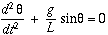
Assuming damping to be in place with a damping coefficient (`b`), we can write the equation as:

`(d^2theta)/dt^2 + (b/m)*(d theta)/dt + (g/L)*sintheta = 0`

The above is a 2nd degree ordinary differential equation which represents the general motion of a pendulum. There are 2 possible configurations of simple pendulums possible:

1). Simple harmonic motion: In this type of configuration, we assume the angle made by the string of the pendulum to be small enough for us to use small angle approximation (`sintheta = theta`). In that case, we do not need to solve the differential equation in order to get various paramters of the pendulum like angular frequency and time period.

The motion equation of the pendulum in this case becomes:
`(d^2theta)/dt^2 + (g/L)*theta = 0`
`omega = sqrt(g/L)`
`T = 2*pi*sqrt(L/g)`

2). Real/Non-linear pendulum: In this case, the angular displacement is large enough for us to not be able to use the small angle approximtion, thus we need to solve the ODE in order to get the various paramters of the pendulum. The ODE does not have a closed form solution, thus we need to solve it numerically with the help of MATLAB.

Assume `theta` to be any random angle `underset(1)(theta)`.
Let `underset(2)(theta) = (d underset(1)(theta))/dt`
`(d^2underset(1)(theta))/dt^2 = (d underset(2)(theta))/dt`

Essentially, `underset(1)(theta)` represents the angular displacement of the pendulum from its mean position and `underset(2)(theta)` represents the angular velocity of the pendulum bob.

With this, we get 2 first order ODEs:

`(d underset(1)(theta))/dt = underset(2)(theta)`
`(d underset(2)(theta))/dt + (b/m)*underset(2)(theta) + (g/L)*sin underset(1)(theta) = 0`

Our solution matrix will be:

`[[(d underset(1)(theta))/dt] , [(d underset(2)(theta))/dt]] = [[underset(2)(theta),0],[-(b/m)*underset(2)(theta),-(g/L)*sin underset(1)(theta)]]`

We then, will have to integrate this solution matrix in order to get the values of angular velocities and displacement.

The following input parameters are taken for the code:
Damping coefficient (`b`) = 0.1 Ns/m
Gravitational acceleration (`g`) = 9.81 m/s2
Length of pendulum string (`L`) = 1 m
Mass of bob (`m`) = 1kg

The initial and mean position of the pendulum is when the bob string is vertical and the bob has an initial velocity of 3rad/s about the pendulum hinge.

Initial Angular displacement = 0 Radians
Initial angular velocity = 3 rad/s

We need to simulate the motion of the pendulum for a total of 20 seconds, during which there will be 500 time stamps (discrete function) at which the MATLAB program will solve the ODE for the values of angular displacement and velocity.

The pendulum hinge, about which the string and bob oscillates, has coordinates set at the origin.

In this program, we will be making use of a source code which helps in solving the two required first order ODEs and gives us the result of the angular displacement and the velocity at each of the 500 time stamps. The source code is as follows:

function [dtheta_dt] = ode_function(t,theta,b,g,l,m)
theta1 = theta(1)%1st value of theta1 (angular displacement)
theta2 = theta(2)%value of theta2
dtheta1_dt = theta2;
dtheta2_dt = -(b/m)*theta2 - (g/l)*sin(theta1) %theta1 is considered in radians
dtheta_dt = [dtheta1_dt;dtheta2_dt]
end

We will be making use of the inbuilt solver ode45 which takes the source code from the function and outputs the angular displacement and velocity.

As output, we will have 2 matrices:
1). t (1x500) matrix: this matrix contains all the 500 time stamps within 0-20 seconds
2). results (2x500) matrix: this matrix contains all the five hundred values of both angular velocity and angular displacement for each time stamp.

Now, at each angular displacement point, we need to find out the coordinates of the bob in order to plot the movement of the pendulum. For this we will be using a 'for' loop going inputing values from the angular displacement column of the results matrix.

By simple trigonometry, we can find out the coordinates of the bob for any random value of angular displacement `theta`:
X-Coordinate of bob = `underset(o)(X) + L*sintheta`
Y-Coordinate of bob = `underset(o)(Y) - L*costheta`
`underset(o)(X)` and `underset(o)(Y)` are the X and Y coordinates of the hinge.

For each value of angular displacement, we will be plotting the lines joining the hinge coordinates and the bob coordinates and we will also be highlighting the bob with a red circular mark and the hinge with a red square mark.

%simple pendullum
%input parameters
%damping coefficient
b = 0.1;
%gravity
g = 9.81;
%length of string
l = 1;
%mass of bob
m = 1;

%initial conditions
theta_0 = [0;3]; %initial angular displacement is 0 rad and intial angular velocity is 5rad/s

%time points/instants
t_span = linspace(0,20,500);

%solving the ODE
[t,results] = ode45(@(t,theta) ode_function(t,theta,b,g,l,m), t_span, theta_0)%function which returns the value of t and results

%hinge coordinates
x0 = 0;
y0 = 0;

ct = 1; %ct represents each frame/configuration of the pendullum
for i = 1:length(t_span)
    %angle which the pendullum string makes with the vertical
    angle = results(i,1);
    %bob coordinates
    x = x0 + l*sin(angle); 
    y = y0 - l*cos(angle);
    %plotting the hinge coordinates x0,yo and bob coordinates x,y and
    %joining to make string
    %hinge represented by square marker, bob represented by circular marker
    plot([x0 x],[y0 y],x0,y0,'s',x,y,'o','markers',10,'markerface','r')
    axis([-2 2 -2 2])
    pause(0.05)
    xlabel('X-AXIS')
    ylabel('Y-AXIS')
    M(ct) = getframe(gcf) %storing each frame in the array M
    ct = ct+1; %moving to the next frame
end

Since we want to animate the simulation, we need to make a video file (.avi) which stores each configuration (each angular displacement) of the pendulum and makes a movie to showcase it in form of an animation. All the configurations of the pendulum will be stored in an array called M with the help of getframe command. The code for the same is given below:

%for generating the video of the pendullum animation
videofile = VideoWriter('Simple Pendullum.avi','Uncompressed AVI')
open(videofile)
writeVideo(videofile,M)
close(videofile)

The ouput pendulum simulation comes out as:

The simulation video link is given below:

Youtube Link

If we want to plot the angular displacement and the velocity of the pendulum, we can do so by the following code:

%plotting angular displacement and angular velocity variations against time
figure(2)
hold on
q = plot(t,results(:,1),'-*');
p = plot(t,results(:,2),'-*');
xlabel('TIME')
ylabel('PLOT')
legend([q p],'Angular Displacement','Angular Velocity')

ERRORS AND PROBLEMS FACED:

1). The first iteration of the program written included the following code for plotting the pendulum string and bob.

%plotting the hinge coordinates x0,yo and bob coordinates x,y and
    %joining to make string
    %hinge represented by square marker, bob represented by circular marker
    hold on
    plot (x,y,'o','markers',10,'markerface','r')
    plot([x0 x],[y0 y])
    axis([-2 2 -2 2])
    pause(0.05)
    xlabel('X-AXIS')
    ylabel('Y-AXIS')
    ct = ct+1; %moving to the next frame

The above code produces a simulation as follows:

Wrong Simulation

2). Another code for plotting which is problematic is given as follows:

%plotting the hinge coordinates x0,yo and bob coordinates x,y and
    %joining to make string
    %hinge represented by square marker, bob represented by circular marker
    plot(x,y,[x0 x],[y0 y],'o','markers',10,'markerface','r')
    axis([-2 2 -2 2])
    pause(0.05)
    xlabel('X-AXIS')
    ylabel('Y-AXIS')
    ct = ct+1; %moving to the next frame

The above code gives the following output:

In the above code, we can write '-o' instead of just 'o' and we will be able to get the pendulum simulation. Thus, this becomes an alternative plotting code.

 %plotting the hinge coordinates x0,yo and bob coordinates x,y and
    %joining to make string
    %hinge represented by square marker, bob represented by circular marker
    plot(x,y,[x0 x],[y0 y],'-o','markers',10,'markerface','r')
    axis([-2 2 -2 2])
    pause(0.05)
    xlabel('X-AXIS')
    ylabel('Y-AXIS')
    ct = ct+1; %moving to the next frame

The full code with appropriate comments is given below:

clear all
close all
clc
%simple pendullum
%input parameters
%damping coefficient
b = 0.1;
%gravity
g = 9.81;
%length of string
l = 1;
%mass of bob
m = 1;

%initial conditions
theta_0 = [0;3]; %initial angular displacement is 0 rad and intial angular velocity is 5rad/s

%time points/instants
t_span = linspace(0,20,500);

%solving the ODE
[t,results] = ode45(@(t,theta) ode_function(t,theta,b,g,l,m), t_span, theta_0)%function which returns the value of t and results

%hinge coordinates
x0 = 0;
y0 = 0;

ct = 1; %ct represents each frame/configuration of the pendullum
for i = 1:length(t_span)
    %angle which the pendullum string makes with the vertical
    angle = results(i,1);
    %bob coordinates
    x = x0 + l*sin(angle); 
    y = y0 - l*cos(angle);
    %plotting the hinge coordinates x0,yo and bob coordinates x,y and
    %joining to make string
    %hinge represented by square marker, bob represented by circular marker
    plot([x0 x],[y0 y],x0,y0,'s',x,y,'o','markers',10,'markerface','r')
    axis([-2 2 -2 2])
    pause(0.05)
    xlabel('X-AXIS')
    ylabel('Y-AXIS')
    M(ct) = getframe(gcf) %storing each frame in the array M
    ct = ct+1; %moving to the next frame
end
%for generating the video of the pendullum animation
videofile = VideoWriter('Simple Pendullum.avi','Uncompressed AVI')
open(videofile)
writeVideo(videofile,M)
close(videofile)

%plotting angular displacement and angular velocity variations against time
figure(2)
hold on
q = plot(t,results(:,1),'-*');
p = plot(t,results(:,2),'-*');
xlabel('TIME')
ylabel('PLOT')
legend([q p],'Angular Displacement','Angular Velocity')