SIMULATION OF SIMPLE PENDULUM CORRESPONDING TO SECOND ORDER ODE WITH MATLAB

SIMPLE PENDULUM

Aim:

Create Simulation of Simple pendulum With MATLAB as solution for second order ODE

Objectives:

Write a program that solves ODE which represents the equation of motion of a simple pendulum with damping

Given Details

Simulate the motion between 0-20 sec

for angular displacement = 0

angular velocity=3 rad/sec

at time t = 0

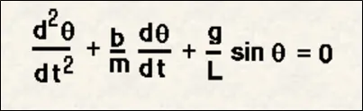
In the above equation,

g = gravity in m/s²

L = length of the pendulum in m

m = mass of the ball in kg

b=damping coefficient

Given Dimensions

L = 1 metre

M = 1 kg

b = 0.05

g = 9.81 m/s²

Theory

A heavy body suspended by a light inextensible thread is called simple pendulum. This is impracticable, so in practice a small metal sphere is suspended from a rigid support using a cotton or silk thread. The point from which the bob is suspended is called point of suspension. The centre of gravity of the bob is called centre of oscillations. The distance between point of suspension and the centre of oscillations is called length of the pendulum.

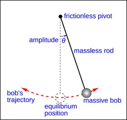
The weight of the bob acts vertically downwards and the tension in the string acts vertically upwards. These two forces are equal and opposite and the bob has equilibrium position in between. The bob displaced by θ angle from equilibrium position.

code for ode45 function call used in main program

function [dtheta_dt]= ode_func(t,theta,b,l,m,g)
theta1=theta(1);
theta2=theta(2);

dtheta1= theta2;
dtheta2=((-b/m).*theta2)-((g/l).*sin(theta1));

dtheta_dt = [dtheta1;dtheta2];

end

MAIN PROGRAM

clear all
close all
clc

b = 0.05;
m =1;
l =1;
g =9.81;

t_span =linspace(0,20,500);
theta_0=[0;3];
[t, results] = ode45(@(t,theta) ode_func(t,theta,b,l,m,g),t_span,theta_0);

figure(1)
plot(t,results(:,1))
hold on
plot(t,results(:,2))
xlabel('Time')
ylabel('Velocity')
legend('displacement','Angular velocity')
hold off

disp = results(:,1);
vel=results(:,2);

%fixed coordinates
x0=0;
y0=-0.1;
ct=1;

for i = 1:length(disp)
    
    %coordinates
    x1=l*cos(disp(i)-pi/2);
    y1=l*sin(disp(i)-pi/2);
    
     %plotting fixed end
     plot([-1.5 1.5],[0 0],'linewidth',25,'color','k')
     hold on 
     %plotting the bob
     plot (x1,y1,'-O','markersize',25,'markerfacecolor','b')
     %joining the end points of line and fixed end
     plot(x0,y0, '-O','markersize',5,'markerfacecolor','k');
     %line connecting the fixed end and bob
     plot ([x0 x1],[y0 y1],'g','linewidth',2)
     %axis setting
     axis([-1.5 1.5 -1.5 1.5])
     
     M(ct)= getframe(gcf);
     ct=ct+1;
     hold off
end
movie(M)                                                                %for creating animation video
videofile=VideoWriter('simple pendulum.avi','uncompressed AVI');
open(videofile)                                                         %open the videofile while running the code
writeVideo(videofile,M)                                                 %for writing the video file
close(videofile)                                                        %for closing the videofile after code run

EXPLANATION OF THE CODE

Firstly, the given details are assigned as variables in the code. Then time span of the simple pendulum is set by using linspace command then theta value is given as a column matrix. After this we use ode45 function and corresponding “ode_fuc” function call in main program. Ode45 is a solver used in MATLAB has much accurate value.

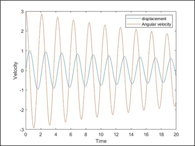
Then used plot command to plot graph corresponding to time and velocity,legend command is used for identify each values in the graph.

For getting the accurate simulation of the simple pendulum corresponding to the second order ODE with damping we need to use the looping statements, here for loop is used to create this.

The pendulum has fixed coordinates mentioned as x0,y0 and x1, y1 are the other coordinates.

Marker command is used for making bob of the pendulum. The axis is fixed using axis command. The counter command is used to make the value changes in each for loop. Then videoWriter command is used to create the video file.

ERROR FACED

1.

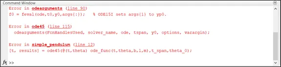
The error faced in using ode45 function call, where the order of each value that depends is not same as in the main program hence error occurred and rectified by arranging the order.

2.

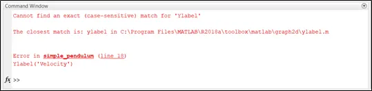
MATLAB is case sensitive, used ‘Ylabel’ should be like ‘ylabel’

RESULTS

· Plot Obtained between Velocity & Time

S SIMULATION OF SIMPLE PENDULUM YOUTUBE

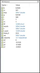
workspace

CONCLUSION

Using MATLAB, Simulation of a Simple Pendulum corresponding to the solution of a Second order ODE is created

REFERANCE

[1] WIKIPEDIA

[2] MATLAB DOCUMENTATION

[3] NCERT PHYSICS TEXT

[4] GOGLE IMAGES