Air Methane mixture combustion simulation using ANSYS Fluent

ANSYS Fluent offers a variety of combustion simulations models. They are classified as follows:

Based on mixing:

Premixed combustion:

Here, the air and fuel mixture is well mixed before combustion starts to take place. e.g., Port fuel injection simulation and simulation where the input is already mixed fuel and air.

Non-premixed combustion:

This model of combustion is utilised when the air and the fuel are not mixed at all before combustion. Diesel engine simulation and late injection fall under this case.

Partially premixed combustion:

In this combustion model, air and fuel mixture is neither fully mixed nor unmixed. This model is used for simulting early combustion where the combustion occurs before the air fuel mixture gets fully mixed.

Based on the place of combustion:

Fluid phase: When combustion takes place on the fluid phase/domain also known as volumetric combustion

Wall : Here, the combustion takes place on the wall/surface.

Particles: In this combustion model, surface reactions occurs on surface of other particles. e.g., cold combustion.

Porous : When reaction take place on a porous region (where there is pressure drop across the region) e.g., after treatment systems.

Based on production rate:

Finite rate chemistry model: Chemical kinetics is used for calculating the production rate of each species. This constitutes a seperate ODE system so finite rate chemistry model is accurate but quite expensive computationally. e.g., used for detailed study of spray models.

Eddy dissipation model: Here, based on turbulent quantities mixing time scale is calculated. After time has passed the mixing time scale, the combustion is said to be completed. The product species are produced instantaneously. e.g., used in simulating burners.

Finite rate chemistry with eddy dissipation model: The short comings of the eddy dissipation model are overcome here. Unlike eddy dissipation models the product species are not produced instantaneously,finite rate chemistry is applied to calculate the rate of production. e.g., used in finding ignition delay

In this project, combustion of air plus methane mixture in burner is demonstrated using Eddy dissipation model. The axisymmetric simulation of the burner is carried out. The 2D geometry of the model is attached below:

The zoomed view of geometry showcasing the fuel inlet:

The mesh of the geometry is shown below:

The size of mesh is selected as 1mm (0.001m) with curve proximity enabled having number of cells across gap set as 3.

The number of nodes of the mesh is: 68326

The number of nodes of the mesh is:67422

Zoomed in view of the mesh:

A steady state axisymmetrical simulation is carried out here with energy equation turned on and using k-epsilon for turbulence modelling. Species transport equation is enabled with volumetric reactions, inlet diffusion and diffusion energy source. Mixture is selected as air+methane with eddy dissipation model.The boundary conditions are taken as follows:

Air-inlet: Inflow boundary with velocity taken as 0.5m/s with turbulent intensity 10% and turbulent length scale as 0.44m. Temperature is taken as 300k with mass fraction of o2 taken as 0.23.

This mass fraction is obtained from the following balanced equation:
`CH_4 + 2O_2 + 7.52N_2 rarr CO_2 + 2H_2O + 7.52N_2`

Fuel-inlet: This is also a inflow boundary with velocity 80m/s with turbulent intensity 10% and hydraulic diameter as 0.01m. Temperature is taken as 300k with mass fraction of ch4 taken as 1.

Outlet: This boundary is assigned as pressure outlet.

Walls and wall-side: Assigned as wall boundary.

Axis: This is the boundary assigned as axis to enable axisymmetry simulation.

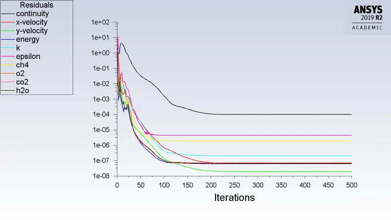
After setting up boundaries, equidistant lines were created using surface option for capturing data at various places. Then, temperature contour is set up and animated for review of the simulation. After that the solution is initialised using hybrid method and run till the residuals stopped changing and reported steady values.

The converge plot of the simulation:

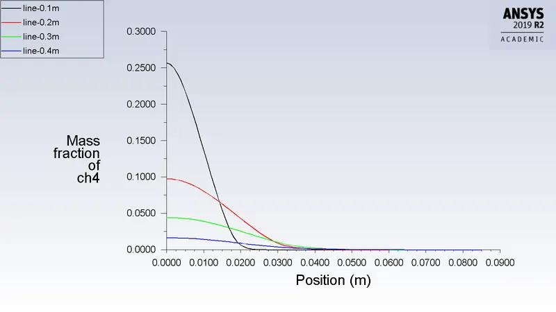
Mass fraction of CH4 at various equidistant line probes:

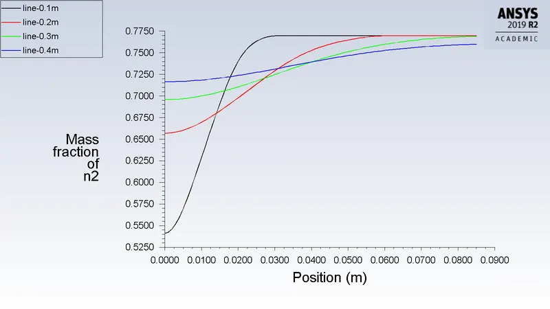
Mass fraction of N2 at various equidistant line probes:

Mass fraction of O2 at various equidistant line probes:

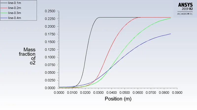
We can see from the above plots that the mass fraction of the ch4,o2 and n2 decreases as we move away from the inlet, this is because the more we move away form the inlet, the more the fuel and air mix together, this leads to combustion as we are using the eddy dissipation model for the simulation. Since ch4, o2 and n2 are the reactants they keep reducing as we move farther. Also we can observe from the ch4 plot that as height increases, the ch4 decreases it is because of the fuel-inlet being present near the bottom of the geometry whereas it the opposite for the o2 and n2. For visual reference, contour image of ch4,o2 and n2 mass fraction are also provided below:

Contour image of mass fraction of ch4:

Contour image of mass fraction of n2:

Contour image of mass fraction of o2:

Products of simulation:

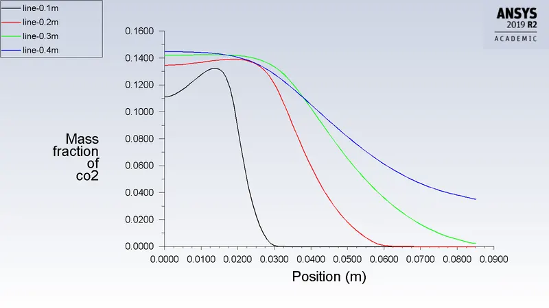
Mass fraction of Co2 at various equidistant line probes:

Mass fraction of H2O at various equidistant line probes:

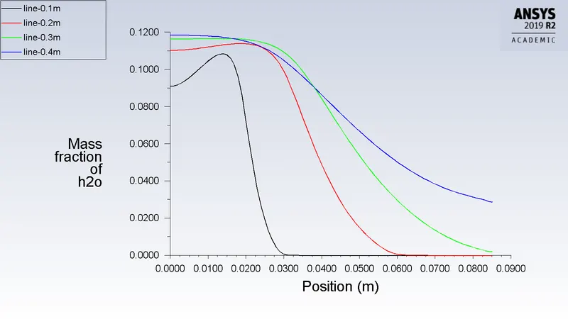
From the above plots of co2 and h2o which are products of the combustion, the mass fraction increases as we move away from the inlet because as we move along the length the mixture will go from unmixed to completely mixed. And as the height increases these products' mass fraction will be less as the distance form combustion increases. For visual representation the contour plots of the co2 and h2o are given below:

Contour image of mass fraction of co2:

Contour image of mass fraction of h2o:

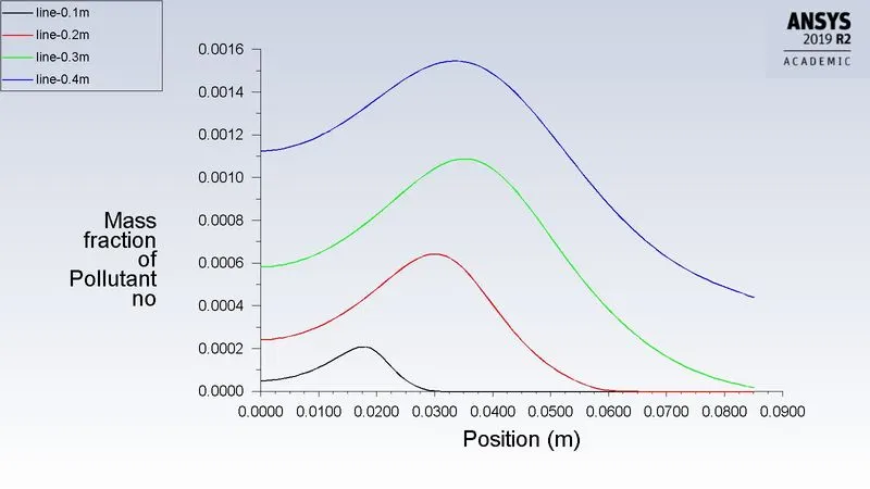
Since formation of NO is very less and has negligible impact on combustion simulation, NO is simulated in postprocessing type mode where after the NO simulation is modelled after the above simulation is conducted. Thermal NOx and Prompt NOx prediction are enabled for the simulation with fuel species taken as ch4. Temperature PDF mode is selected for the simulation. Then after setting up the NOx model, equations except NO and temperature variance equations, other equations are turned off and the simulation is continued for another 50 iterations. From the simulation the follwing plot and contour image is obtained.

Mass fraction of pollutant NOx at various equidistant line probes:

Contour image of mass fraction of pollutant no:

Contour image of temperature:

Animation of the temperature contour: (showing the simulation attaining the steady state)