Steel surface defect detection project: classify NEU images with Python
One complete machine vision project on the NEU hot-rolled steel images, run end to end by Skill-Lync: hand-made texture features against a pretrained CNN, the split that makes every model look perfect, an honest batch test, a lighting check and the full code.
By Skill-Lync · Published 19 Nov 2026 · Every number below was produced by the code on this page (scikit-learn 1.9.1, onnxruntime 1.32.0, CPU only)
What is a steel surface defect detection project?
It is a model that looks at a camera image of a steel strip and names the defect on it: a scratch, a patch, an inclusion and so on. Steel mills run cameras over strip moving at several metres per second, and no inspector can watch every metre. Think of the model as a second inspector who never blinks, but has only seen the images you trained it on.
On the NEU images, both of our models scored 99.3% or better on the random split most tutorials use. Trained on the first 210 images of each class and tested on the last 90, the texture model fell to 91.5%, while a pretrained ResNet-18 held 97.0%. The second test is the one that looks like a factory: the model meets images it was not built around.
What is in the NEU surface defect database?
1,800 greyscale photos of hot-rolled steel strip, each 200 × 200 pixels, 300 for each of six defect types. Kechen Song and Yunhui Yan's group at Northeastern University, China, publish it free. NEU-CLS has one label per image for classification; NEU-DET adds boxes around each defect for detection.
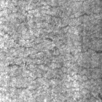
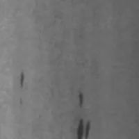
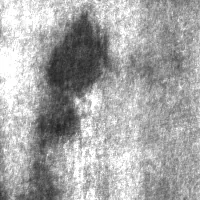

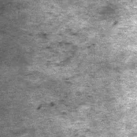
One image per class from NEU-CLS (files Cr_1, In_2, Pa_1, PS_1, RS_1 and Sc_1), shown unaltered. Source: NEU surface defect database, Kechen Song, Northeastern University (checked 19 Nov 2026). The authors ask users to cite their papers: K. Song and Y. Yan, Applied Surface Science 285 (2013) 858-864, and, for NEU-DET, Y. He, K. Song, Q. Meng and Y. Yan, IEEE Transactions on Instrumentation and Measurement 69(4) (2020) 1493-1504, which reports 74.8 and 82.3 mAP for its detector.
The database page itself names the two difficulties. Defects of one class look very different (a scratch can be horizontal, vertical or slanting), while rolled-in scale, crazing and pitted surface look alike. And the brightness changes with lighting and material. Keep the second one in mind: it decides the results below.
A trap in the download. NEU-CLS comes as an old RAR archive. macOS's built-in tools and bsdtar extract it without an error, but most of the files come out corrupt ("cannot identify image file"). Use real unrar, 7-Zip or pip install unrar-cffi, then check that all 1,800 files open.
Which features describe a steel surface?
Two kinds, compared here on the same images. Texture features are hand-made rules that count small patterns in the pixels. A pretrained CNN turns each image into 512 numbers it learned from millions of everyday photos. A simple classifier then learns which numbers mean which defect.
- Texture + SVM (88 numbers). Local binary patterns (LBP): every pixel is compared with its neighbours on a circle and the up/down pattern is counted, at three circle sizes. Think of it as a fingerprint of the surface's grain. Plus grey-level co-occurrence (GLCM) statistics, which measure how often a dark pixel sits next to a bright one, and the image's mean and spread of brightness. A support vector machine (SVM) classifies them.
- ResNet-18 + logistic regression (512 numbers). A ResNet-18 trained on the ImageNet photo collection, frozen, with its last layer cut off. Each steel image is resized to 224 × 224 and copied into three colour channels, and the network's 512 pooled outputs become the features. This is transfer learning without any training of the network: no GPU, no fine-tuning.
LBP itself ignores overall brightness, since it only compares each pixel with its neighbours. The brightness enters through the GLCM statistics and the mean and spread, and that turns out to matter.
Why do most NEU projects report 99% accuracy?
Because a random split hands the model near-copies of its test images. NEU's images are numbered 1 to 300 within each class, and neighbours in that numbering look alike. Split at random and almost every test image has a close sibling in training. Holding out a block of numbers removes most of those siblings.
100.0%
97.0%
97.2%
94.1%
The evidence for the siblings: in texture-feature space, an image's nearest neighbour sits within five numbers of it 41.6% of the time, against about 3.3% if the order were random (median distance 10 numbers). NEU does not document how the images were numbered, so we cannot say they are crops of the same coil. We can say the order is not random, and a random split ignores it.
Five-fold cross-validation tells the same story. Shuffled folds gave the texture model 98.9, 100, 98.6, 99.4, 98.9% (mean 99.2%). Folds of 60 consecutive numbers gave 94.4, 95, 99.4, 99.2, 98.9% (mean 97.4%): the first two blocks are the hard ones. The CNN barely moved: 99.7% shuffled, 99.4% in blocks.
Where does the texture model go wrong?
Almost all its errors are one defect: inclusions. Of the 90 later-batch inclusion images it named only 49 correctly, calling 29 of them "pitted surface" and 12 "scratches". The other five classes were near-perfect. The CNN got 75 of the inclusions right and still lost 14 to pitted surface.
| True ↓ / predicted → | Cr | In | Pa | PS | RS | Sc | Recall |
|---|---|---|---|---|---|---|---|
| Crazing | 90 | 0 | 0 | 0 | 0 | 0 | 100.0% |
| Inclusion | 0 | 49 | 0 | 29 | 0 | 12 | 54.4% |
| Patches | 1 | 0 | 89 | 0 | 0 | 0 | 98.9% |
| Pitted surface | 0 | 1 | 0 | 89 | 0 | 0 | 98.9% |
| Rolled-in scale | 0 | 0 | 0 | 0 | 90 | 0 | 100.0% |
| Scratches | 0 | 3 | 0 | 0 | 0 | 87 | 96.7% |
Texture + SVM, trained on images 1-210 of each class, tested on images 211-300 (90 per class). Rows are the truth, columns the prediction. Cr crazing, In inclusion, Pa patches, PS pitted surface, RS rolled-in scale, Sc scratches.
The clue is brightness. The average grey level of each class drifts along the numbering, and the later inclusion images are lighter than the earlier ones:
| Mean grey level (0-255) | 1-60 | 61-120 | 121-180 | 181-240 | 241-300 |
|---|---|---|---|---|---|
| Crazing | 140 | 127 | 131 | 144 | 163 |
| Inclusion | 94 | 96 | 100 | 118 | 124 |
| Patches | 156 | 132 | 119 | 121 | 135 |
| Pitted surface | 186 | 178 | 184 | 167 | 168 |
| Rolled-in scale | 138 | 127 | 136 | 104 | 84 |
| Scratches | 118 | 112 | 90 | 72 | 84 |
Inclusions average 94-100 in the first 180 images and 118-124 after that, moving towards pitted surface, the brightest class. A model that leans on brightness and contrast will drift with them. Rolled-in scale darkens even more, from 138 to 84, but its texture is distinctive enough that the model still got all of it right.
Is it only brightness? We re-ran the texture model on images with their brightness normalised (each image scaled to zero mean and unit spread, mean and spread dropped from the features). Later-batch accuracy rose from 91.5% to 93.0%: better, but still behind the CNN. The rest is a change in the defects' look, and pretrained features cope with it better.
What happens when the lighting changes?
We darkened and brightened the later-batch images by 20% (pixel values times 0.8 or 1.2, clipped at white) without retraining. The texture model dropped to 90.0% and 86.3%. The CNN stayed at 97.2% and 94.1%. Brighter hurts both more, because the lightest pixels saturate and their texture is lost.
A lamp ageing, a dirty lens cover or a new coil grade can shift brightness this much on a real line. That is why inspection systems fix their lighting, and why a test on deliberately altered images belongs in any defect project you show an interviewer.
How many labelled images do you need?
With pretrained features, very few. Using only 10 labelled images per defect, the CNN averaged 95.7% on the later batch (range 93.3-97.6% over 10 random draws). The texture model needed all 210 per defect to reach 91.5%. For a plant building its own dataset, that is a far smaller labelling job.
The texture model's curve flattens around 91%: more images from the same early batch do not fix features that shift between batches. The CNN gains little past 50 per class. In both cases, more variety in the training images (other coils, shifts and lamps) is worth more than more of the same.
The full Python code
About 80 lines of NumPy, scikit-image, scikit-learn and ONNX Runtime. Put the NEU-CLS folder and resnet18-v1-7.onnx next to the script and run it. It prints the accuracies and confusion matrices behind the ladder and tables above in about four minutes on a laptop CPU.
# Steel surface defect classification on the NEU-CLS images (1,800 greyscale 200 x 200 px, 6 defects).
# Put the NEU-CLS folder (Cr_1.bmp ... Sc_300.bmp) and resnet18-v1-7.onnx (ONNX Model Zoo) next to this
# script. Needs numpy, pillow, scikit-image, scikit-learn, onnx, onnxruntime. No GPU needed.
import numpy as np, onnx, onnxruntime as ort
from PIL import Image
from skimage.feature import local_binary_pattern, graycomatrix, graycoprops
from sklearn.svm import SVC
from sklearn.linear_model import LogisticRegression
from sklearn.preprocessing import StandardScaler
from sklearn.pipeline import make_pipeline
from sklearn.model_selection import train_test_split
from sklearn.metrics import confusion_matrix

CLASSES = ["Cr", "In", "Pa", "PS", "RS", "Sc"]  # crazing, inclusion, patches, pitted surface, rolled-in scale, scratches
imgs = np.array([np.array(Image.open(f"NEU-CLS/{c}_{i}.bmp")) for c in CLASSES for i in range(1, 301)])
y = np.repeat(np.arange(6), 300)                 # class label
num = np.tile(np.arange(1, 301), 6)              # image number within its class, 1-300

def texture(a):  # hand-made texture features: LBP histograms at 3 scales + GLCM statistics + brightness
    f = []
    for P, R in [(8, 1), (16, 2), (24, 3)]:
        lbp = local_binary_pattern(a, P, R, "uniform")
        f += list(np.histogram(lbp, bins=P + 2, range=(0, P + 2), density=True)[0])
    g = graycomatrix(a // 8, [1, 3], [0, np.pi / 4, np.pi / 2, 3 * np.pi / 4], levels=32, symmetric=True, normed=True)
    for p in ["contrast", "homogeneity", "energy", "correlation"]:
        f += list(graycoprops(g, p).ravel())
    return f + [a.mean(), a.std()]

# Transfer learning: a ResNet-18 trained on ImageNet, frozen, used as a 512-number feature extractor.
net = onnx.load("resnet18-v1-7.onnx")
net.graph.output.append(onnx.helper.make_tensor_value_info("flatten_170", onnx.TensorProto.FLOAT, None))
sess = ort.InferenceSession(net.SerializeToString(), providers=["CPUExecutionProvider"])
MEAN = np.array([0.485, 0.456, 0.406], np.float32)[:, None, None]
STD = np.array([0.229, 0.224, 0.225], np.float32)[:, None, None]

def cnn(batch):  # grey 200 x 200 -> RGB 224 x 224, ImageNet normalisation, 50 images at a time
    out = []
    for b in range(0, len(batch), 50):
        x = [np.array(Image.fromarray(a).resize((224, 224), Image.BILINEAR), np.float32)[None] / 255 for a in batch[b:b + 50]]
        out.append(sess.run(["flatten_170"], {"data": (np.repeat(np.stack(x), 3, 1) - MEAN) / STD})[0])
    return np.concatenate(out)

T = np.array([texture(a) for a in imgs])
F = cnn(imgs)
svm = lambda: make_pipeline(StandardScaler(), SVC(C=10, gamma="scale"))
logreg = lambda: make_pipeline(StandardScaler(), LogisticRegression(C=0.1, max_iter=3000))
MODELS = {"Texture + SVM": (T, svm), "ResNet-18 + logistic regression": (F, logreg)}

def fit_score(name, tr, te):
    X, make = MODELS[name]
    p = make().fit(X[tr], y[tr]).predict(X[te])
    return (p == y[te]).mean(), confusion_matrix(y[te], p, labels=range(6))

# 1. The usual split: 70/30 at random. Images that sit next to each other in the numbering
#    look alike, so near-copies of many test images are in the training set.
tr, te = train_test_split(np.arange(1800), test_size=0.3, stratify=y, random_state=42)
for name in MODELS:
    print(f"Random 70/30 split, {name}: {fit_score(name, tr, te)[0]:.1%}")

# 2. A later batch: train on images 1-210 of every class, test on 211-300 (same 70/30 sizes).
late = num > 210
for name in MODELS:
    acc, cm = fit_score(name, ~late, late)
    print(f"Later batch, {name}: {acc:.1%}")
    print(cm)

# 3. Lighting check: the later batch again, 20% darker and 20% brighter (clipped at 255).
for gain in (0.8, 1.2):
    dimmed = np.clip(imgs[late] * gain, 0, 255).astype(np.uint8)
    feats = {"Texture + SVM": np.array([texture(a) for a in dimmed]), "ResNet-18 + logistic regression": cnn(dimmed)}
    for name, (X, make) in MODELS.items():
        acc = (make().fit(X[~late], y[~late]).predict(feats[name]) == y[late]).mean()
        print(f"Later batch at {gain:.0%} light, {name}: {acc:.1%}")
This is the same file we ran to produce the numbers on this page. Install with pip install numpy pillow scikit-image scikit-learn onnx onnxruntime (we used NumPy 2.5.5, scikit-image 0.26.0, scikit-learn 1.9.1, ONNX Runtime 1.32.0). The model file is resnet18-v1-7.onnx from the ONNX Model Zoo (validated/vision/classification/resnet, Apache 2.0 licence): ResNet-18 v1 trained on ImageNet (ILSVRC 2012) in MXNet Gluon, 69.93% top-1 on ImageNet. The learning curve and cross-validation numbers come from a second script that imports this one.
How do you make this project stand out?
Report the later-batch number, not the 99%, and show the inclusion errors with their brightness drift. Then fix the cause rather than adding layers: normalise brightness, train with brightness changes added on purpose, and test on lighting you did not train on.
- Augment the lighting. Add copies of the training images at random brightness and contrast, then rerun the 80% and 120% light tests. The gap between them is your robustness score.
- Fine-tune the CNN. Unfreeze the last ResNet block and train it on NEU with a small learning rate. Compare against the frozen features on the later batch, not the random split.
- Go from "what" to "where". Move to NEU-DET and train a detector (YOLO, Faster R-CNN) that draws a box around each defect. Report mean average precision per class, and check which defects it misses.
- A second dataset. Test on another public steel set, such as the Severstal steel defect detection images on Kaggle (a 2019 competition, labelled with pixel masks). Expect a drop and explain it.
The honest limits of this project
Small, clean crops. Each NEU image is a 200 × 200 crop with the defect in it. A real line camera sees mostly defect-free steel, so the hard problem is finding the rare defect in hours of clean strip and keeping false alarms low. NEU has no "no defect" class at all.
Our later batch is a stand-in. NEU does not say how its images were numbered or when they were taken. The block test removes near-copies; it is not proof of a new production run. Use per-coil or per-day splits when your own data has them.
One run, one seed. The headline accuracies come from one split each; only the learning curve averages 10 draws. With 90 test images per class, one image is 0.2 percentage points of the overall accuracy, so read differences under a point as noise.
What to learn to build projects like this
Python with NumPy for images as arrays, the basics of image processing (filters, edges, texture, segmentation), then machine learning: classifiers, cross-validation and honest evaluation. CNNs and transfer learning come after that. Skill-Lync's Basics of Computer Vision using Python and Advanced Deep Learning using Python courses cover this in 12 weeks each, ₹40,000 each.
- Basics of Computer Vision using Python: image processing, edge detection, segmentation and features, matching, and ML-based vision techniques.
- Advanced Deep Learning using Python: neural networks, optimisers, model evaluation and two weeks on convolutional neural networks.
- Sister projects with the same leakage lesson: bearing fault detection on CWRU vibration data and jet-engine remaining life on NASA C-MAPSS.
- Computer vision courses in India, compared, and all Skill-Lync AI and ML courses with fees.
FAQs
Is the NEU surface defect dataset good for a final-year project?
Yes. It is free, small (1,800 images of 200 × 200 pixels) and runs on a laptop without a GPU: the full code on this page took about four minutes on a CPU. To stand out, do not stop at the random-split accuracy. Test on a later block of images, check lighting changes and explain the errors.
Why do NEU projects report 99% accuracy?
Because a random split puts near-copies of the test images into training. In NEU, images with nearby numbers look alike: an image's closest look-alike sits within five numbers of it 41.6% of the time, against about 3.3% by chance. Testing on images 211-300 dropped our texture model from 99.3% to 91.5%.
Do I need deep learning for steel surface defect detection?
Not to train one. A ResNet-18 already trained on everyday photos, used only as a feature extractor, with a logistic regression on top, reached 97.0% on the later batch with no GPU and no fine-tuning. Training your own CNN from scratch on 1,800 images is slower and easy to overfit. Start with frozen pretrained features.
What is the difference between NEU-CLS and NEU-DET?
Both use the same six hot-rolled steel defects. NEU-CLS is for classification: one label per 200 × 200 image, 300 images per class. NEU-DET adds bounding boxes that mark where each defect is, for object detection models such as YOLO or Faster R-CNN. This page uses NEU-CLS.
How many labelled images do I need to train a defect classifier?
Fewer than you think with pretrained features. On our later-batch test, 10 images per defect gave 95.7% on average with ResNet-18 features, already above the texture model trained on all 210 per class (91.5%). Collect variety, such as different coils, shifts and lighting, rather than more images of the same coil.