Week 9 - Parametric study on Gate valve.

Aim:

For this challenge, you will have to perform a parametric study on the gate valve simulation by setting the opening from 10 % to 80%.

Objective:

• Obtain the mass flow rates at the outlet for each design point.
• Calculate the flow coefficient and flow factor for each opening and plot the graph.
• Discuss the results of the mass flow rate and flow coefficient.

Theory and Introduction:

A gate valve, also known as a sluice valve, is a valve that opens by lifting a barrier (gate) out of the path of the fluid. Gate valves require very little space along the pipe axis and hardly restrict the flow of fluid when the gate is fully opened. The gate faces can be parallel but are most commonly wedge-shaped (in order to be able to apply pressure on the sealing surface).

Gate valves are used to shut off the flow of liquids rather than for flow regulation, which is frequently done with a globe valve. When fully open, the typical gate valve has no obstruction in the flow path, resulting in very low flow resistance. The size of the open flow path generally varies in a nonlinear manner as the gate is moved. This means that the flow rate does not change evenly with stem travel. Depending on the construction, a partially open gate can vibrate from the fluid flow.

Gate valves are mostly used with larger pipe diameters (from 2" to the largest pipelines) since they are less complex to construct than other types of valves in large sizes.

At high pressures, friction can become a problem. As the gate is pushed against its guiding rail by the pressure of the medium, it becomes harder to operate the valve. Large gate valves are sometimes fitted with a bypass controlled by a smaller valve to be able to reduce the pressure before operating the gate valve itself.

Gate valves without an extra sealing ring on the gate or the seat are used in applications where minor leaking of the valve is not an issue, such as heating circuits or sewer pipes.

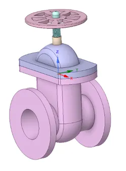
Fig 1. Gate valve

Modelling approach:

Pre-processing:

In pre-processing we first import the geometry in space claim in which we can see there are different parts like bonnet, gate disk, spindle, hand wheel and bottom case. Now here we need to move the gate disk so we disable all the other geometries except the spindle and gate disk. Now we select the move option and select the gate disk using box selection and move it upward 10 mm and then going in group we set the parameter. Now our parameterization group is created. Next we select the pull option and pull both sides till 800mm then we do the volume extract by selecting the edges after volume extraction we supress all the geometry except the volume.

Next we moves to meshing module, in this module we apply the mesh and name the boundaries like inlet and outlet here our mesh is normal but we applies the inflation to outlet as we have to calculate the mass flow rate at outlet so we so the total thickness inflation of 5 mm and then close the mesh module.

Setup:

Solver setup: in solver we set type of solver as pressure based and steady tie solver and here we turn the gravity effect on as we are dealing with gravity so we turn it on at z direction.

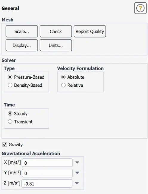
Fig 2. Solver setup

Boundaries setup:

Here we set the inlet boundary as pressure inlet with 10 pa pressure as we are dealing with valve problem.

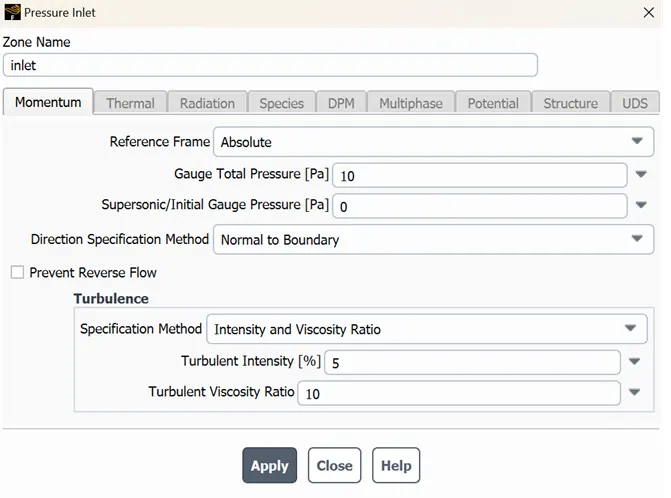
Fig 3. Boundaries setup

Material: as fluid material we are going with water liquid so we take it from fluent database

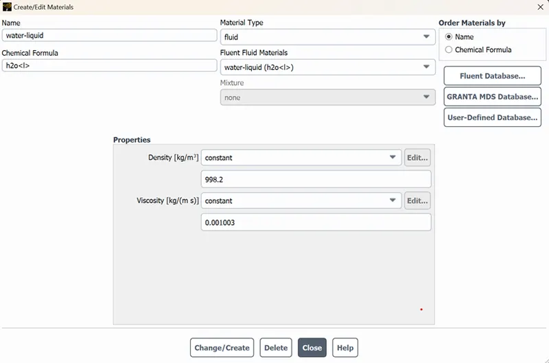
Fig 4. Material selection

Viscous model :

Now to select the viscous model we have to know what is the Reynolds number and what kind of flow it is and for that we need velocity so going In initialization part we can get the inlet velocity which we can see below our velocity is 0.1415488m/s

Reynolds number formula is

Re = (998.2*0.1415*0.1)/0.0010

Re = 14124 so we can clearly say that our flow is turbulent

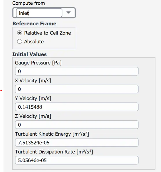
Fig 5. Velocity calculate

As we know the flow type we can set the viscous model so we set it to k-epsilon with scalable wall function.

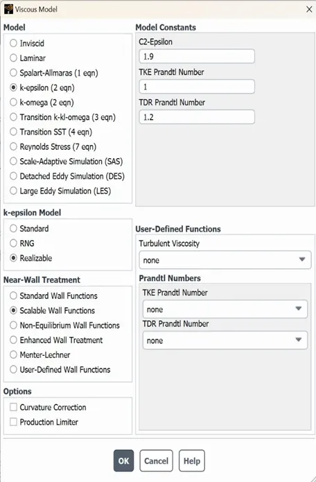
Fig 6. Viscous model

We select coupled method and standard initialization and then run the calculation

Post-processing:

Results

Now going in parameters set we set the values from 10 to 80 mm like 10mm, 20mm, 30mm, 40mm, 50mm, 60mm, 70mm of opening of gate and during setup we take one report definition of mass flow rate in which we set it as parameter, because we want that value to be print in parameter set which we can see in fig below.

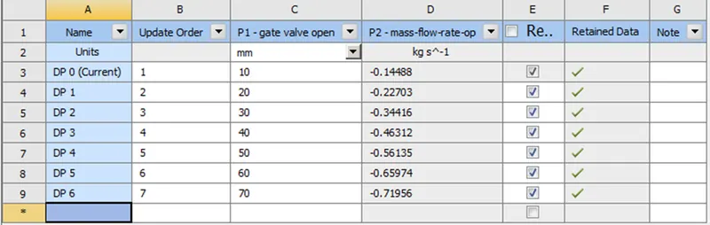
Fig 7. Parameters set

In above fig we can see the mass flow rate is going on increasing as we open the valve gradually. Now we are going to calculate coefficient flow and flow factor using the mass flow rate using the below 2 equations we can calculate both.

Flow coefficient:

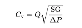
where:

Q is the rate of flow,

SG is the specific gravity of the fluid (for water = 1),

ΔP is the pressure drop across the valve (expressed in pa).

Flow factor:

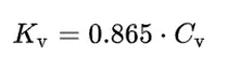
Using above equation and mass flow rate we can calculate flow coefficient and flow factor, we cn see as the valve is opening the mass flow rate is increasing and as the flow increase the flow coefficient and flow factor is also increases we can see it in below table .

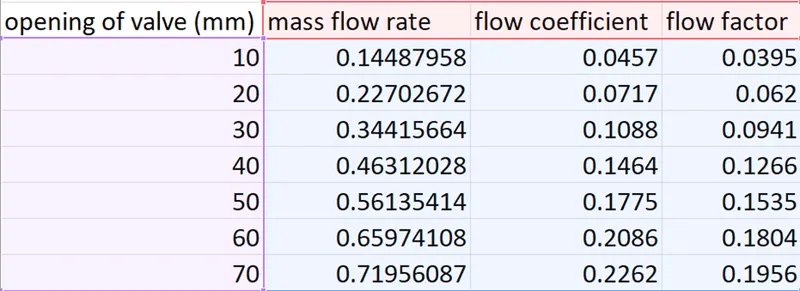
Fig 8. Flow coefficient and flow factor results

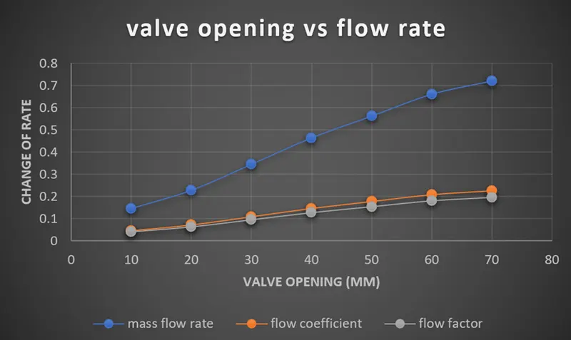
Fig 9. Trend showing chart

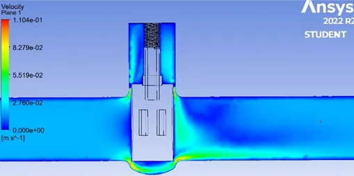
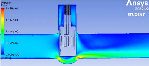
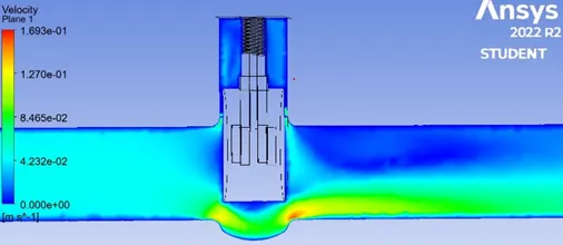
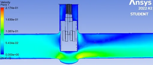
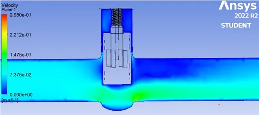
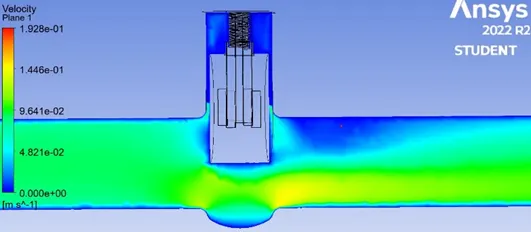
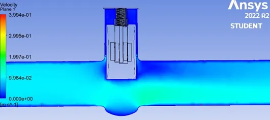
Fig 10. velocity contour and valve opening from 10mm to 70mm

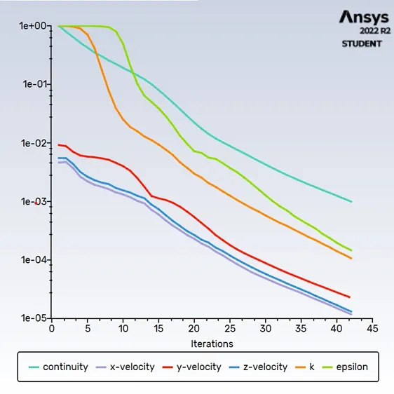
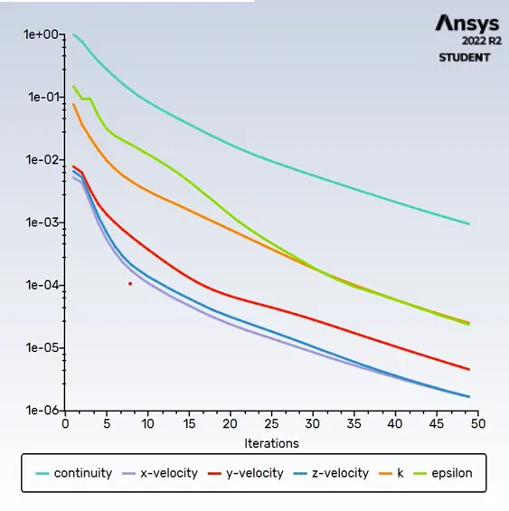
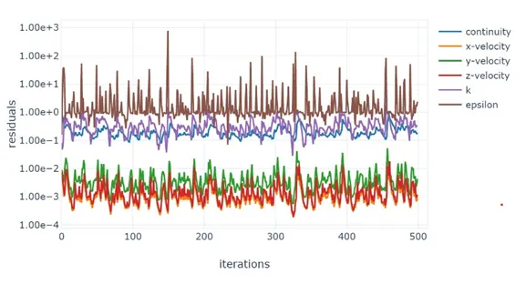
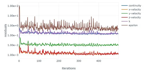
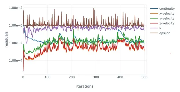
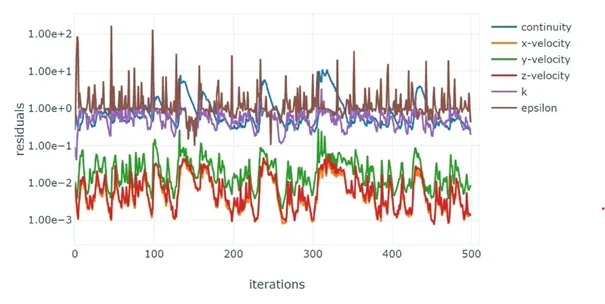
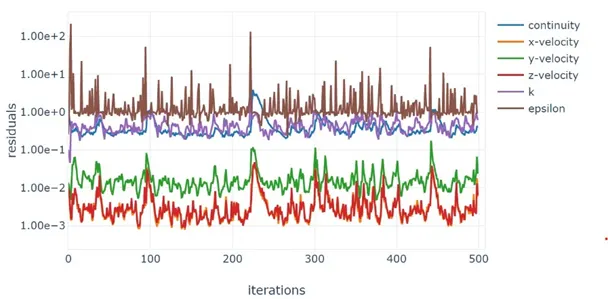
Fig 11. Scaled residuals from 10mm to 70mm

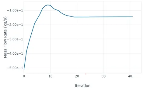
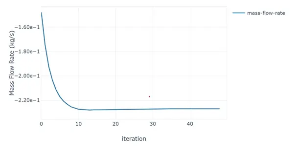
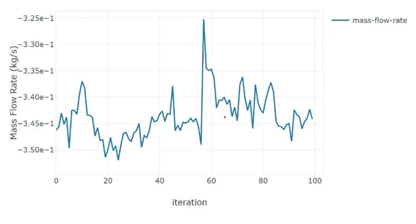
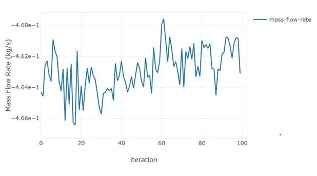
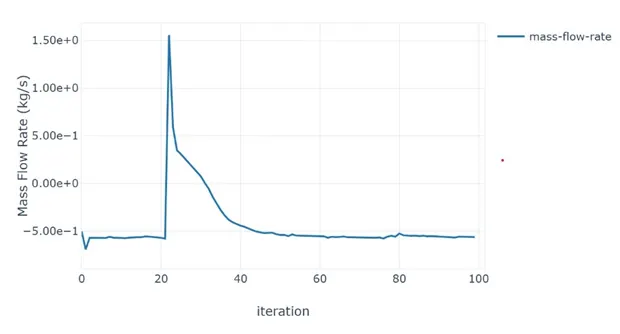
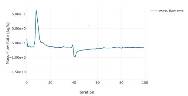
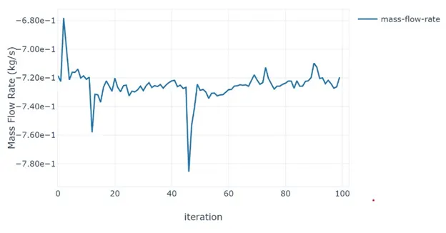
Fig 11. Mass flow rate charts 10mm to 70mm

Conclusion:

Here we can conclude that as we increase the size of opening of valve the mass flow rate is also increases and with increase in mass flow rate the flow coefficient and flow factors are also increases gradually.