Week 9 - Parametric study on Gate valve.
AIM:- To perform a parametric study on a gate valve simulation by setting the opening from 10 % to 80%.
OBJECTIVE:-
1.To simulate the flow of fluid through a gate valve.
2.To obtain the mass flow rates at the outlet for each design point.
3.To calculate the flow coefficient and flow factor for each opening and plot the graph.
4.Discuss the results of the mass flow rate and flow coefficient.
DESCRIPTION:-
A Gate valve also known as sluice valve is a valve that opens by lifting a barrier (gate) out of the path of the fluid. Gate valves require very little space along the pipe axis and hardly restict the flow of fluid when the gate is fully opened. The gate faces can be parallel but are most commonly wedge-shaped in order to be able to apply the pressure on the sealing surface.
Main components of the gate valve are body, seat, stem, bonnet and actuator.The main operation mechanism is very simple.When the hand wheel is turned it rotates the fluid which is translated into the vertical movement of the gate disc via threads.They are considered multi-turn valves as it makes more than one 360 degree turn to fully open/close the valve. When the gate is lifted from the path of the flow,the valve opens and when it returns to its closed position, it seals the bore resulting in a full closure of the valve.
PARAMETRIC STUDY:-
One of the best ways to get value out of yoour simulation is to do parametric analysis with very little marginal work with a model which can be parameterized to simulate scenarios limited only by computational time and resources. As you move forward in your design you can access the impact that is changing the certain parameters accordingly to the design criteria.The parameters can include dimensional parameters. Parametricc studies sllow you to nominate parameters for evaluation, define the parameter range, specify the design constraints and analyse the results of each parameter variation.
A parametric study requires the following
1.Design objective is set to parametric dimensions.
2.Parameters nominated for use in the simulation
3.Design criteria specified
4.Various configurations generated.
FLOW COEFFICIENT:-
The flow coefficient of a device is relative measure of its efficiency at allowing fluid flow.It describes the relationship between the pressure drop across an orifice valve or other assembly and the corresponding flow rate. Mathematically the flow coefficient or flow capacity rating Cv can be expressed as
Cv=Q√SGΔPCv=QSGΔP
Where Q is the rate of flow (gallons per minute)
SG is the specific gravity of fluid (for water =1)
ΔPΔP is the pressure drop across the valve expressed in psi.
10 Pa = 0.00145038 psi
The use of flow coefficient offers a standard method of comparing valve capacities and sizing valves for specific applications that are widely accepted by the industry.The general definition of the flow coefficient can be expanded into equations modelling the flow of liquids, gases and steam using the discharge coefficient.
FLOW FACTOR:-
The metric equivalent factor Kv commonly used in europe and Aisa is calculated using metric units
Kv=Q√SGΔPKv=QSGΔP
Kv can be calculated from Cv using the equation as given below
Kv = 0.865Cv
The Kv factor of the valve indicates, The water flow m3/h at a pressure drop across the valve of 1kgf/cm2 when the valve is completely open.
Opening the space claim and opening the Gate valve model
The model looks as follows
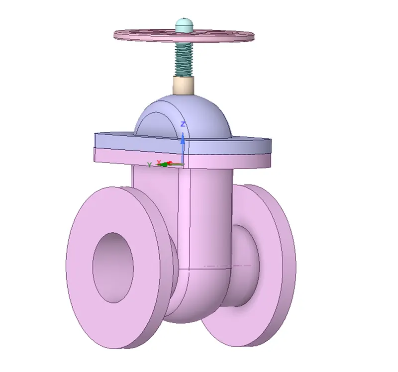
First we will do for the case without parametric study
Now hiding the bottom surface and then gate disc is visible and using move tool with component selection and move the gate disc in upward z direction for 10mm.
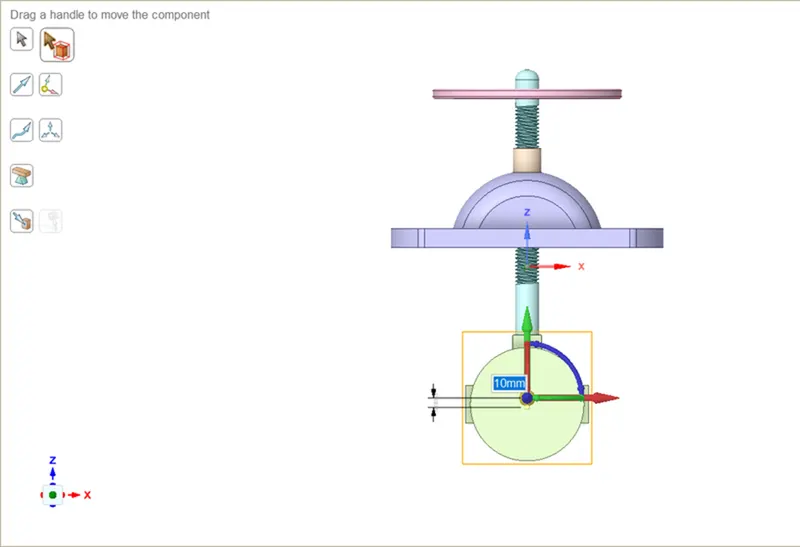
Now extracting the fluid volume from prepare>volume extract>edges select inlet and outlet and part under bonet.
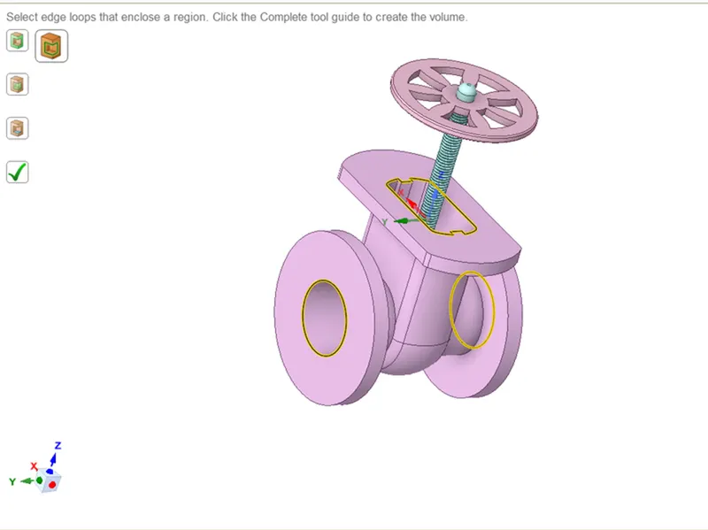
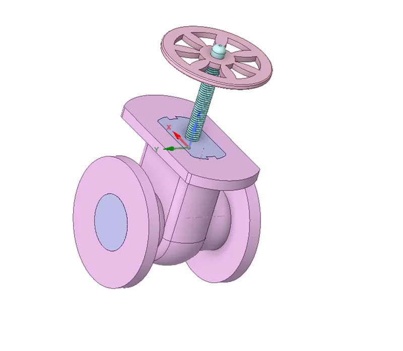
Next using the pull tool pulling the inlet by 800mm and for output also 800mm.
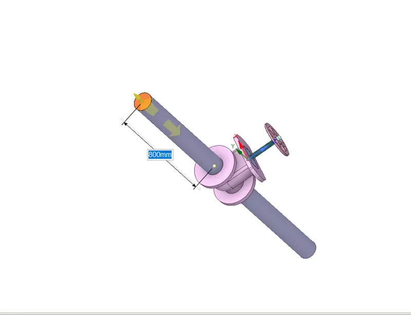
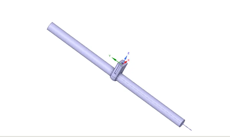
Now going for meshing
Generating a generaal mesh
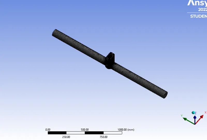
Next is naming the parts.
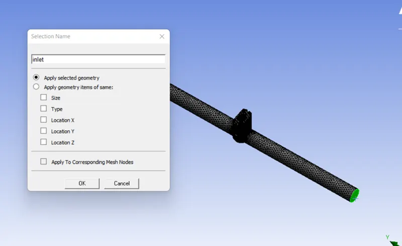
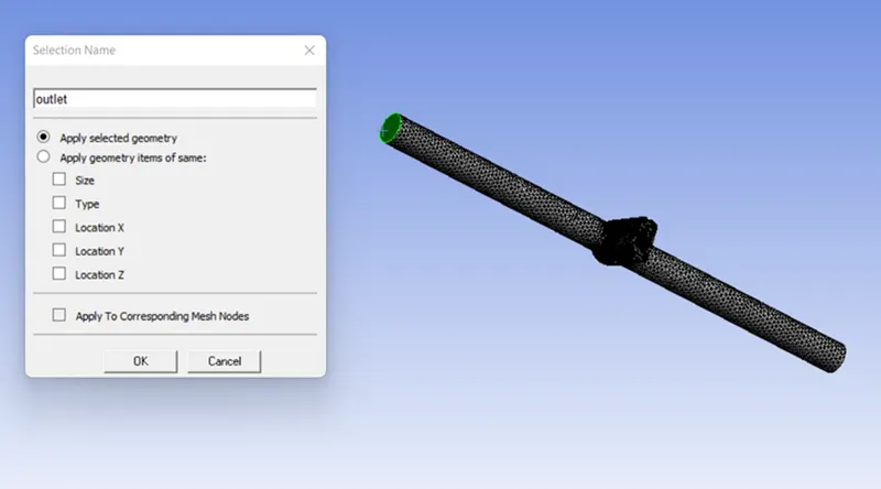
CASE SETUP :
- The following case studies are set for this simulation.
|
GATE VALVE POSITION (in 'mm') |
GAUGE PRESSURE AT INLET (in 'Pa') |
GAUGE PRESSURE AT OUTLET (in 'Pa') |
PRESSURE DIFFERENCE (ΔP)(ΔP) |
||
|
(in 'Pa') |
(in 'bar') |
||||
|
CASE - 1 |
10 |
10 |
0 |
10 |
0.0001 |
|
CASE - 2 |
20 |
10 |
0 |
10 |
0.0001 |
|
CASE - 3 |
30 |
10 |
0 |
10 |
0.0001 |
|
CASE - 4 |
40 |
10 |
0 |
10 |
0.0001 |
|
CASE - 5 |
50 |
10 |
0 |
10 |
0.0001 |
|
CASE - 6 |
60 |
10 |
0 |
10 |
0.0001 |
|
CASE - 7 |
70 |
10 |
0 |
10 |
0.0001 |
|
CASE - 8 |
80 |
10 |
0 |
10 |
0.0001 |
PROCEDURE :
CASE 1 (Gate valve lift - 10mm) :
PRE-PROCESSING :
- Import the given gate valve model into spaceclaim and use the pull tool to extend either sides of the valve pipe to 800mm.
- Make sure that the fluid volume is extracted properly and also the lift of the gate valve is set to 10mm.
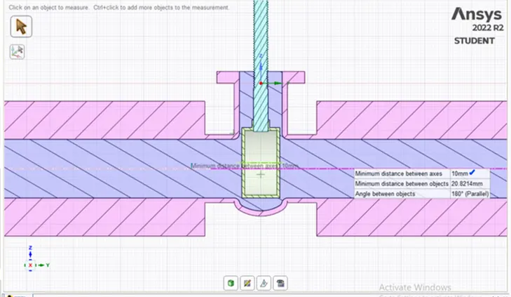
- The inner diameter of the valve pipe in which the fluid is flowing, is measured to be 100mm. So, for 10% to 80% of the gate valve opening, the lift of the gate valve which is given as the input parameter, is to be taken from 10mm to 80mm with 10mm increment. Now, close the spaceclaim.
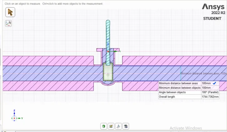
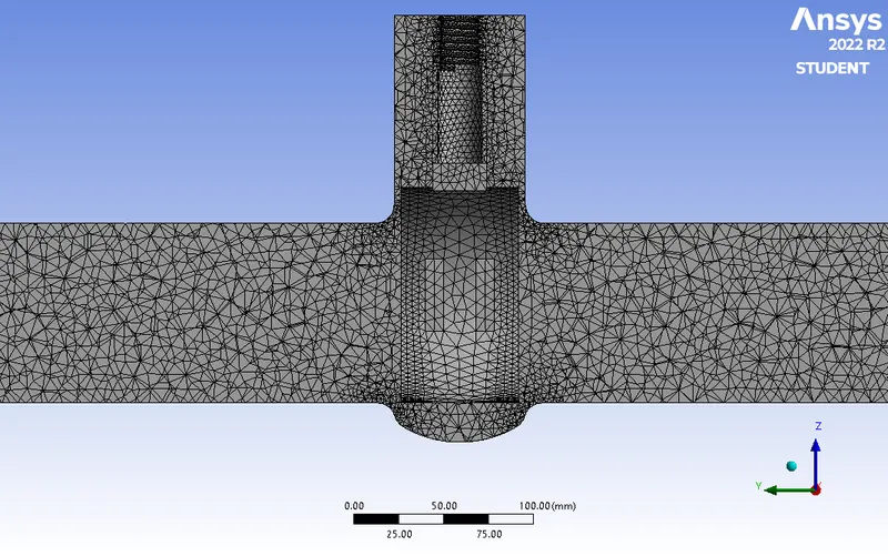
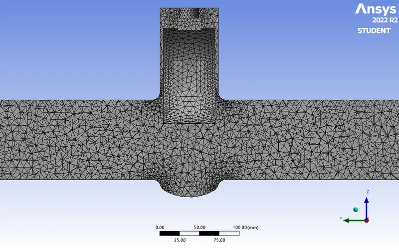
- Open the mesh window and give the required named selections for model. Now, generate the mesh by choosing the mesh element size as 10mm and the maximum mesh size also to be 10mm which generates a uniform mesh.
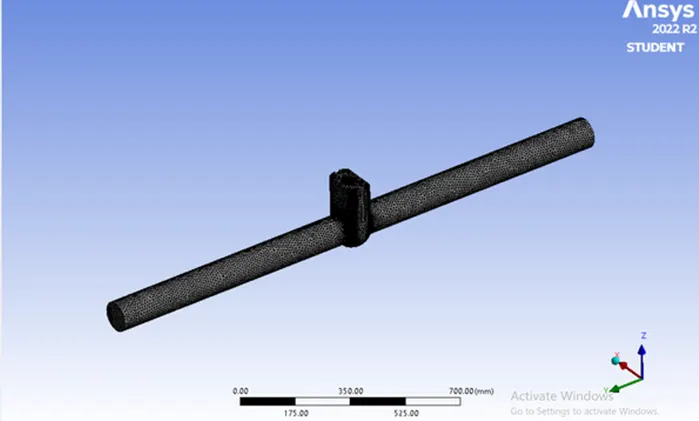
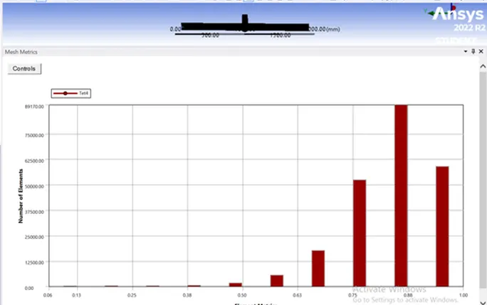
- Since most number of the mesh elements have about 88% of element quality, the mesh quality is good for the simulation.
- Cross sectional view
|
Cells |
Faces |
Nodes |
|
226230 |
468271 |
45834 |
SETUP AND SOLVING :
- Setup the simulation by providing the following input parameters in the setup window.
|
Model |
Settings |
|
Space |
3D |
|
Time |
Steady |
|
Viscous |
RNG k-epsilon turbulence model |
|
Wall Treatment |
Standard Wall Functions |
|
RNG Swirl Dominated Flow Option |
Enabled |
Material properties :
|
Fluid |
water-liquid |
|
Density |
998.2 kg/m^3 |
|
Cp (Specific Heat) |
4182 J/(kg K) |
|
Thermal Conductivity |
0.6 W/(m K) |
|
Viscosity |
0.001003 kg/(m s) |
|
Molecular Weight |
18.0152 kg/kmol |
Boundary conditions :
|
inlet |
|
|
Reference Frame |
Absolute |
|
Gauge Total Pressure [Pa] |
10 |
|
Supersonic/Initial Gauge Pressure [Pa] |
0 |
|
Direction Specification Method |
Normal to Boundary |
|
outlet |
|
Backflow Reference Frame |
Absolute |
|
Gauge Pressure [Pa] |
0 |
|
Backflow Direction Specification Method |
Normal to Boundary |
|
wall-volume_volume |
|
|
Wall Motion |
Stationary Wall |
|
Shear Boundary Condition |
No Slip |
Solution method :
|
Pressure-Velocity Coupling |
Coupled |
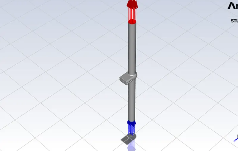
- Here, we enable the gravity having value of 9.81 m/s^2 in negative z-direction since the gravity acts perpendicular to the direction of flow in this setup.
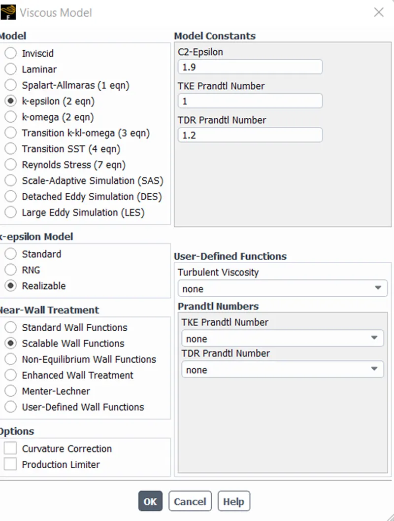
- For this setup, we choose k-epsilon RNG turbulence model with swirl dominated flow option enabled since this visous model will be the better option for incompressible flows having swirling effects.
- Select the fluid material as water from fluent database.
- Make sure the fluid material for the fluid domain cell zone is set to water.
- Set the boundary condition type for inlet as pressure inlet with total gauge pressure of 10 Pa.
- For outlet, select the type as pressure outlet with gauge pressure of 0 Pa (open to atmosphere).
- Create the report definition for mass flow rate at outlet and enable the create parameter option to set it as the output parameter for the simulation.
- Initialize the simulation using hybrid initialization.
- Run the simulation for 500 iterations.
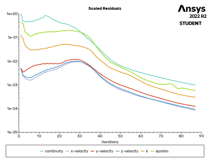
RESIDUALS PLOT :
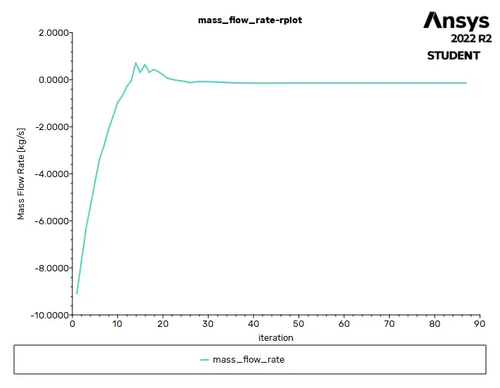
MASS FLOW RATE AT OUTLET PLOT :
Solution status :
- From the above plots, we see that the solution got converged at 87th iteration since the rate at which residuals and mass flow rate at oulet value changes become constant over iteration.
|
Value |
Absolute Criteria |
Convergence Status |
|
|
continuity |
0.0009723831 |
0.001 |
Converged |
|
x-velocity |
8.342491e-05 |
0.001 |
Converged |
|
y-velocity |
0.0001238028 |
0.001 |
Converged |
|
z-velocity |
9.265241e-05 |
0.001 |
Converged |
|
k |
0.000301145 |
0.001 |
Converged |
|
epsilon |
0.0005590986 |
0.001 |
Converged |
Report definitions :
|
mass_flow_rate |
-0.1426206 |
kg/s |
|
Volumetric Flow Rate |
-0.00014287778 |
m^3/s |
POST PROCESSING :
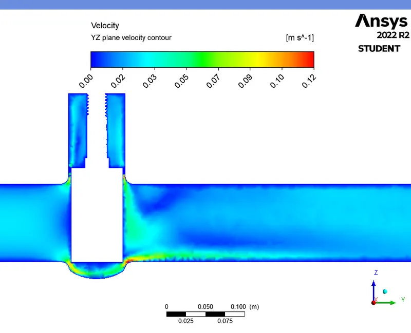
VELOCITY CONTOUR :
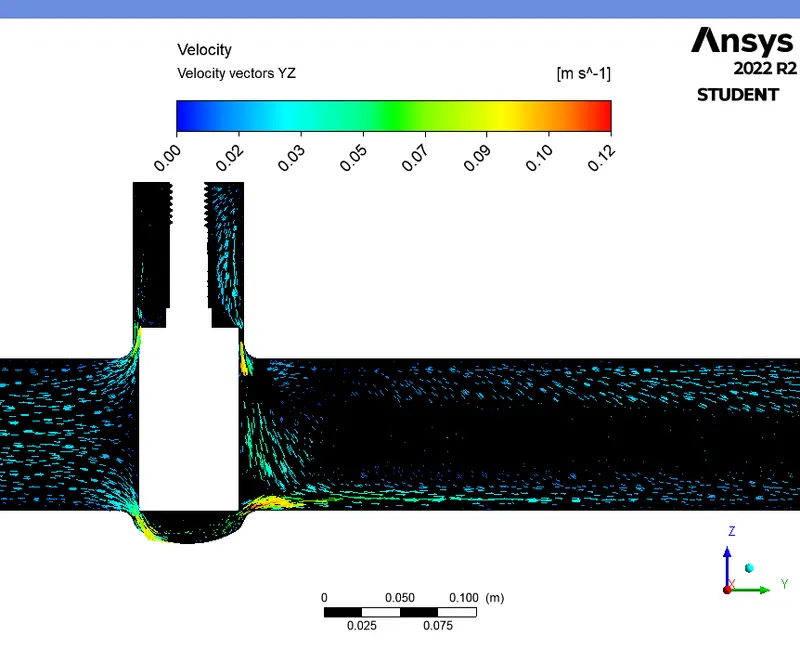
VELOCITY VECTORS :
CASE 2 (Gate valve lift - 20mm) :
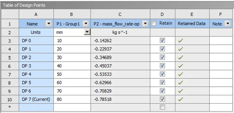
- Create another design point in the Parameter set window from workbench by giving the valve lift value as 20mm under input parameter and update the design point. The fluent will automatically update the geometry, mesh , setup, solution and results for the specified lift value, and also will give the value of mass flow rate at outlet which was set as the output parameter.
PRE-PROCESSING :
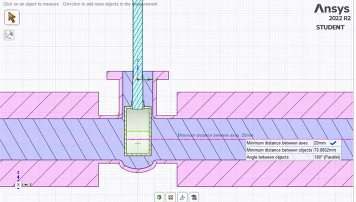
- Cross sectional view of the gate valve with fluid volume.
- Cross sectional view of the mesh elements for the fluid volume.
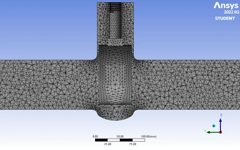
|
Cells |
Faces |
Nodes |
|
224561 |
464568 |
45389 |
RESIDUALS PLOT :
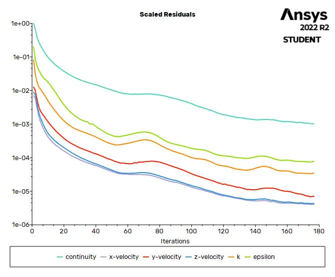
MASS FLOW RATE AT OUTLET PLOT :
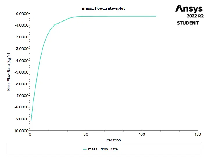
Solution status :
- From the above plots, we see that the solution got converged at 100th iteration since the rate at which residuals and mass flow rate at oulet value changes become constant over iteration.
|
Value |
Absolute Criteria |
Convergence Status |
|
|
continuity |
0.0009978 |
0.001 |
Converged |
|
x-velocity |
4.090286e-06 |
0.001 |
Converged |
|
y-velocity |
6.937372e-06 |
0.001 |
Converged |
|
z-velocity |
4.282387e-06 |
0.001 |
Converged |
|
k |
3.531111e-05 |
0.001 |
Converged |
|
epsilon |
7.813134e-05 |
0.001 |
Converged |
Report definitions :
|
mass_flow_rate |
-0.2293705 |
kg/s |
- The negative sign in the mass flow rate indicates that the fluid is leaving the system.
Calculation of Volumetric flow rate :
We know that,
Volume flow rate (Q) = Mass flow rate / Density of the fluid (water)
Q = 0.2293705/998.2
|
Volumetric Flow Rate |
-0.000229784 |
m^3/s |
POST PROCESSING :
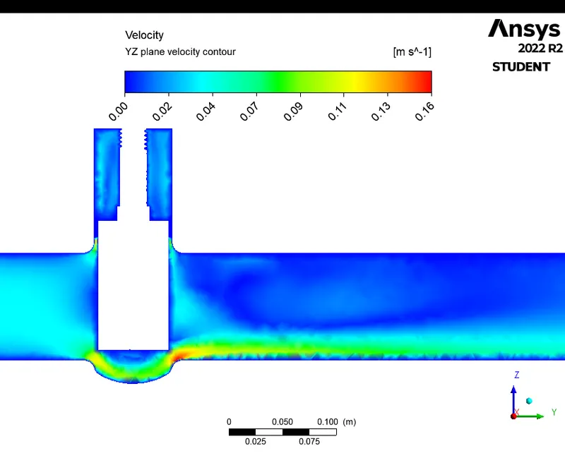
VELOCITY CONTOUR :
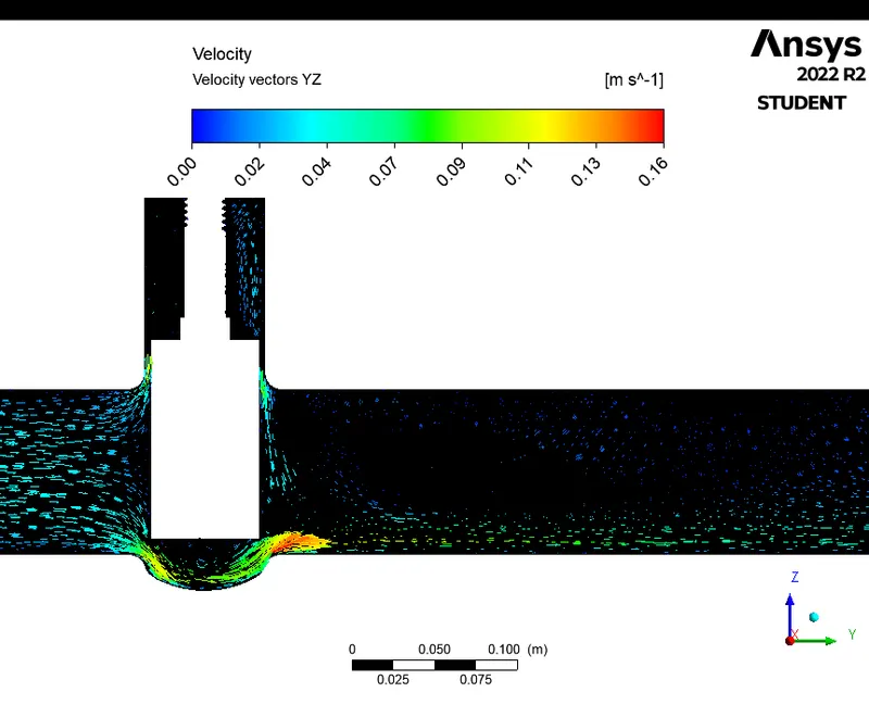
VELOCITY VECTORS :
CASE 3 (Gate valve lift - 30mm) :
- Create another design point in the Parameter set window for lift value of 30mm and update the design point.
PRE-PROCESSING :
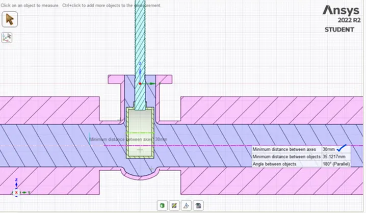
- Cross sectional view of the gate valve with fluid volume.
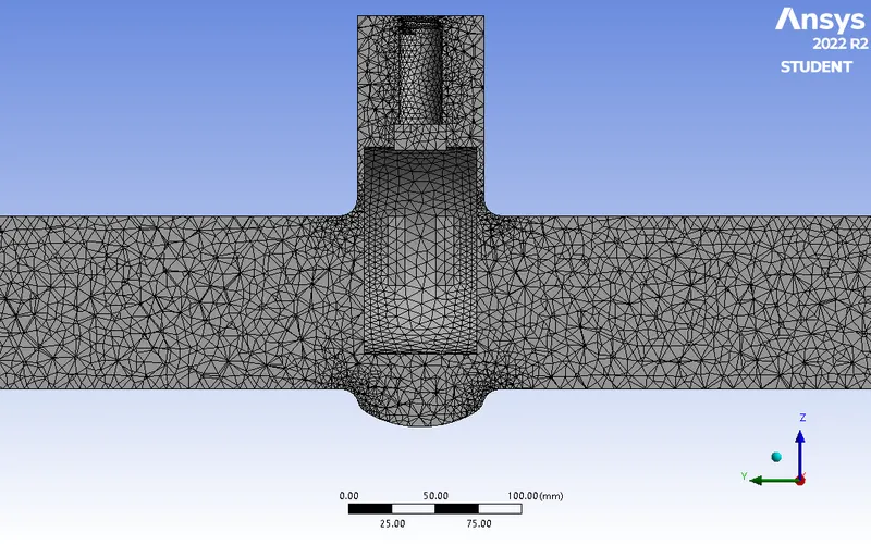
- Cross sectional view of the mesh elements for the fluid volume.
|
Cells |
Faces |
Nodes |
|
222083 |
459284 |
44824 |
RESIDUALS PLOT :
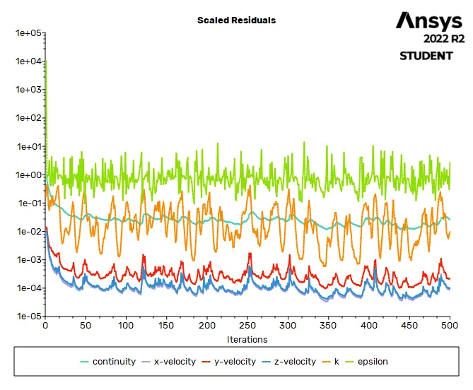
MASS FLOW RATE AT OUTLET PLOT :
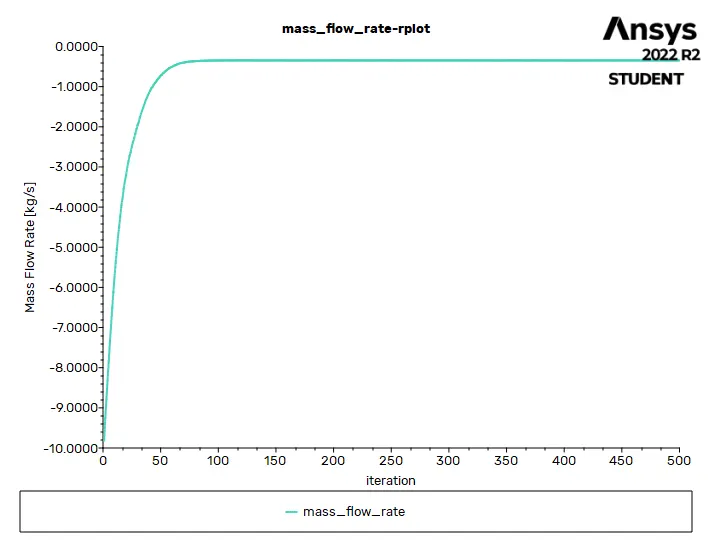
Solution status :
- From the above plots, we see that the solution got converged at 200th iteration since the rate at which residuals and mass flow rate at oulet value changes become constant over iteration.
|
Value |
Absolute Criteria |
Convergence Status |
|
|
continuity |
0.0267538 |
0.001 |
Not Converged |
|
x-velocity |
8.868771e-05 |
0.001 |
Converged |
|
y-velocity |
0.0002176496 |
0.001 |
Converged |
|
z-velocity |
0.0001000305 |
0.001 |
Converged |
|
k |
0.009749514 |
0.001 |
Not Converged |
|
epsilon |
2.738883 |
0.001 |
Not Converged |
Report definitions :
|
mass_flow_rate |
-0.3468929 |
kg/s |
Calculation of Volumetric flow rate :
We know that,
Volume flow rate (Q) = Mass flow rate / Density of the fluid (water)
Q = 0.3468929/998.2
|
Volumetric Flow Rate |
-0.0003475184 |
m^3/s |
POST PROCESSING :-
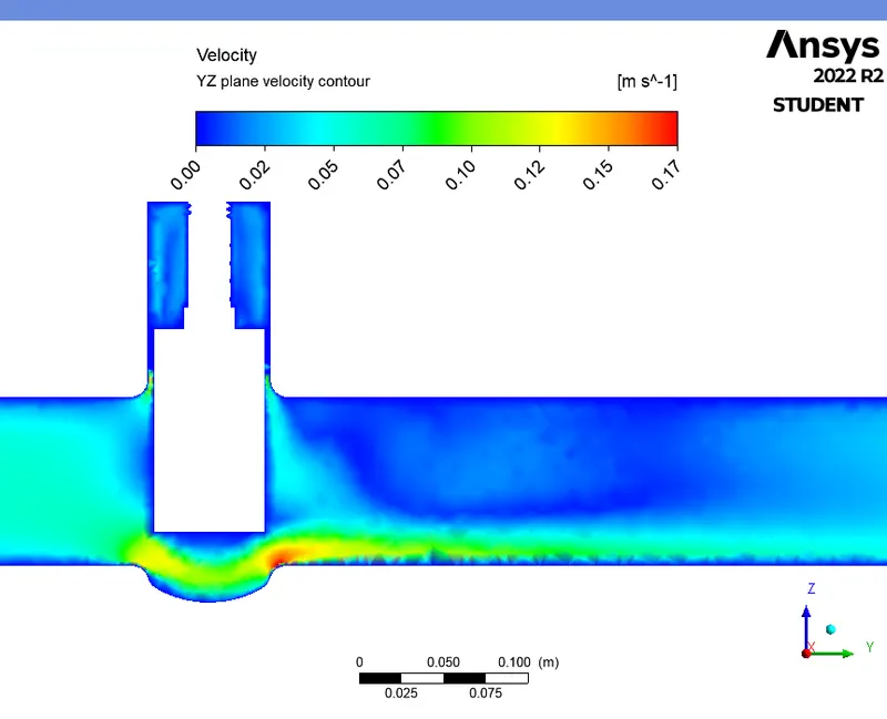
VELOCITY CONTOUR :-
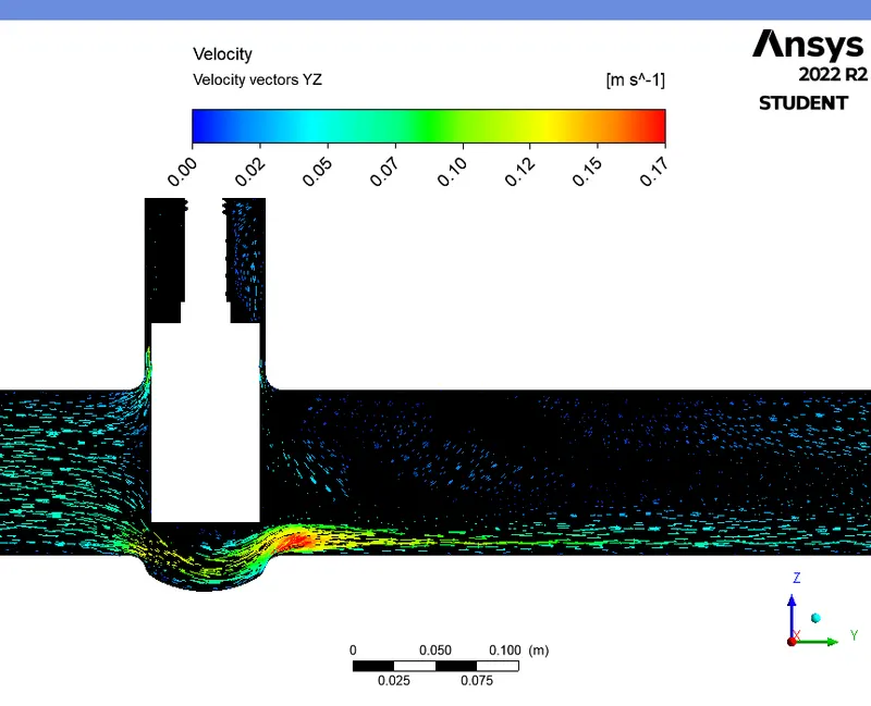
VELOCITY VECTORS :-
CASE 4 (Gate valve lift - 40mm) :-
- Create another design point in the Parameter set window for lift value of 40mm and update the design point.
PRE-PROCESSING :
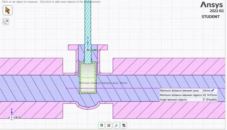
- Cross sectional view of the gate valve with fluid volume.
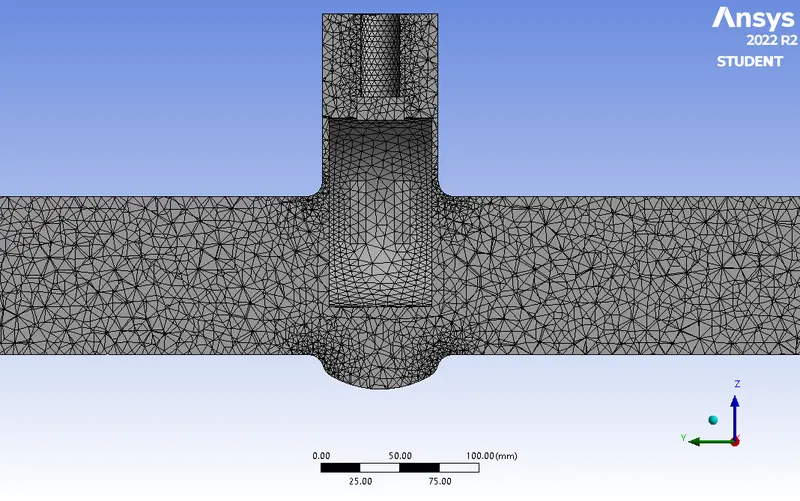
- Cross sectional view of the mesh elements for the fluid volume.
|
Cells |
Faces |
Nodes |
|
219283 |
453406 |
44232 |
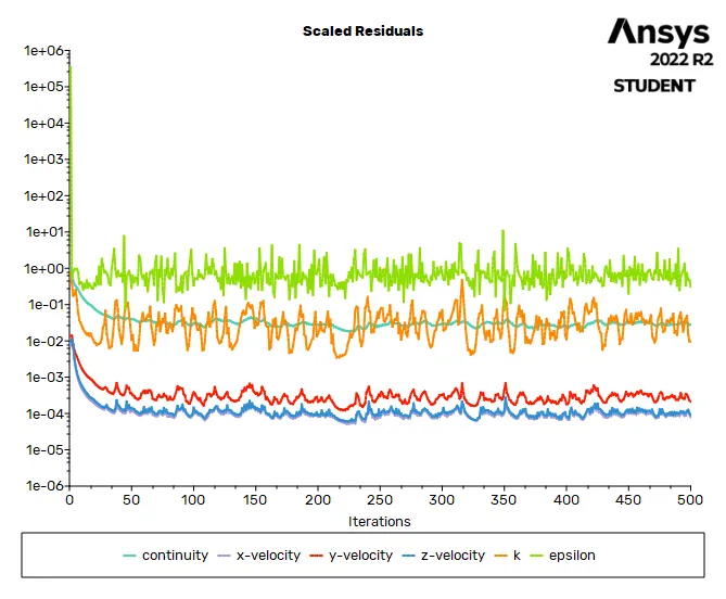
RESIDUALS PLOT :-
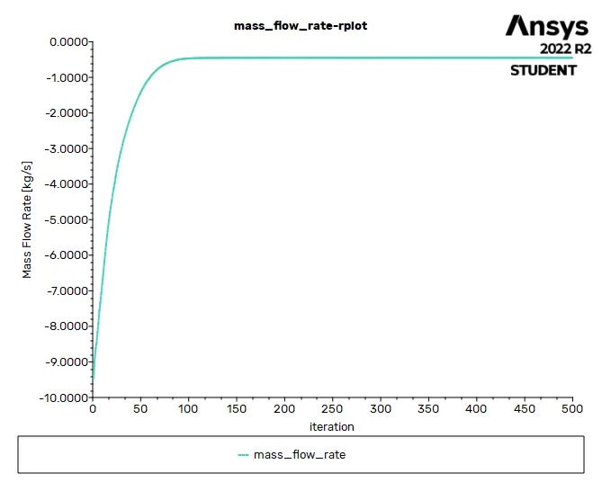
MASS FLOW RATE AT OUTLET - PLOT :-
Solution status :-
- From the above plots, we see that the solution got converged at 200th iteration since the rate at which residuals and mass flow rate at oulet value changes become constant over iteration.
|
Value |
Absolute Criteria |
Convergence Status |
|
|
continuity |
0.02798982 |
0.001 |
Not Converged |
|
x-velocity |
7.86329e-05 |
0.001 |
Converged |
|
y-velocity |
0.0002134795 |
0.001 |
Converged |
|
z-velocity |
9.09735e-05 |
0.001 |
Converged |
|
k |
0.00964965 |
0.001 |
Not Converged |
|
epsilon |
0.3102351 |
0.001 |
Not Converged |
Report definitions :-
|
mass_flow_rate |
-0.4503665 |
kg/s |
Calculation of Volumetric flow rate :-
We know that,
Volume flow rate (Q) = Mass flow rate / Density of the fluid (water)
Q = 0.4503665/998.2
|
Volumetric Flow Rate |
-0.0004511786 |
m^3/s |
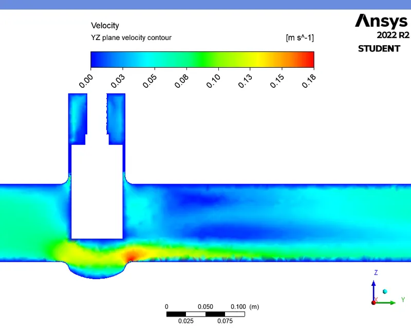
VELOCITY CONTOUR :-
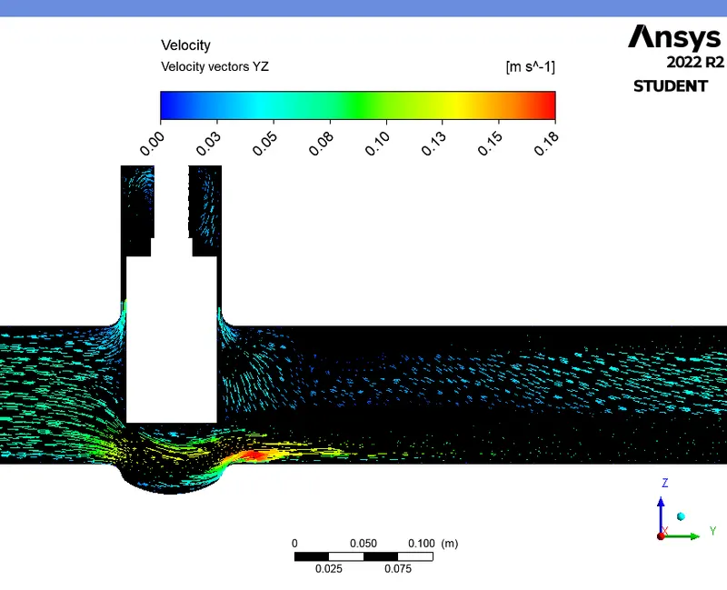
VELOCITY VECTORS :-
CASE 5 (Gate valve lift - 50mm) :-
- Create another design point in the Parameter set window for lift value of 50mm and update the design point.
PRE-PROCESSING :-
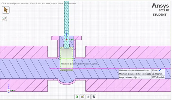
- Cross sectional view of the gate valve with fluid volume.
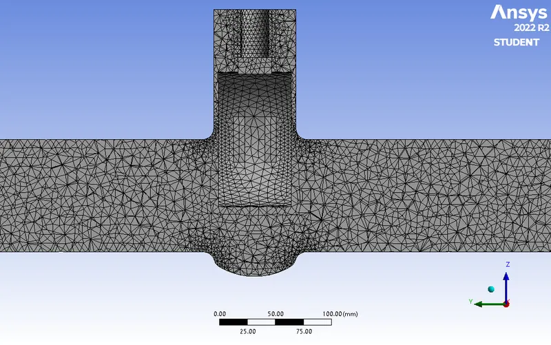
- Cross sectional view of the mesh elements for the fluid volume.
|
Cells |
Faces |
Nodes |
|
218410 |
451550 |
44040 |
RESIDUALS PLOT :-
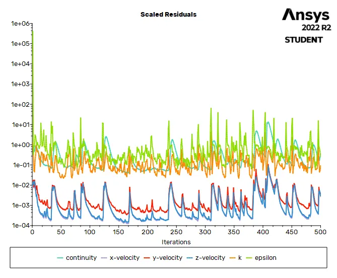
MASS FLOW RATE AT OUTLET - PLOT :-
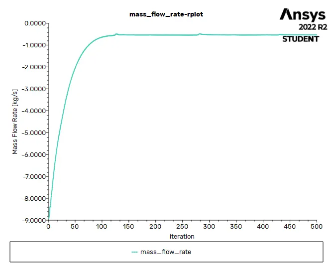
Solution status :-
- From the above plots, we see that the solution got converged at 450th iteration since the rate at which residuals and mass flow rate at oulet value changes become constant over iteration.
|
Value |
Absolute Criteria |
Convergence Status |
|
|
continuity |
0.3740099 |
0.001 |
Not Converged |
|
x-velocity |
0.00269189 |
0.001 |
Not Converged |
|
y-velocity |
0.003484739 |
0.001 |
Not Converged |
|
z-velocity |
0.002710014 |
0.001 |
Not Converged |
|
k |
0.09197593 |
0.001 |
Not Converged |
|
epsilon |
0.2623293 |
0.001 |
Not Converged |
Report definitions :-
|
mass_flow_rate |
-0.5353329 |
kg/s |
Calculation of Volumetric flow rate :-
We know that,
Volume flow rate (Q) = Mass flow rate / Density of the fluid (water)
Q = 0.5353329/998.2
|
Volumetric Flow Rate |
-0.000536298 |
m^3/s |
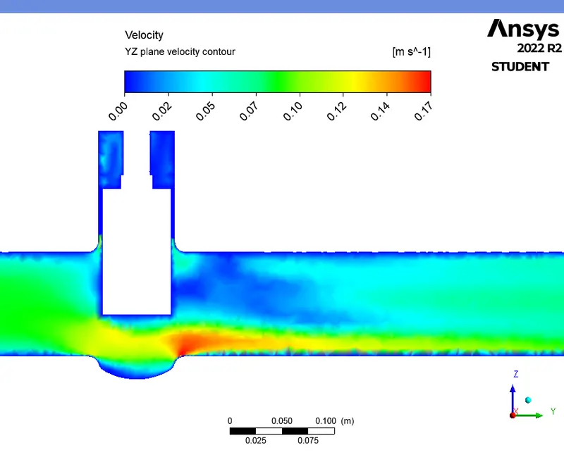
VELOCITY CONTOUR :-
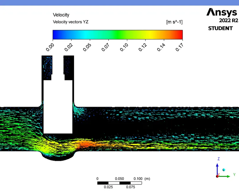
VELOCITY VECTORS :-
CASE 6 (Gate valve lift - 60mm) :
- Create another design point in the Parameter set window for lift value of 60mm and update the design point.
PRE-PROCESSING :
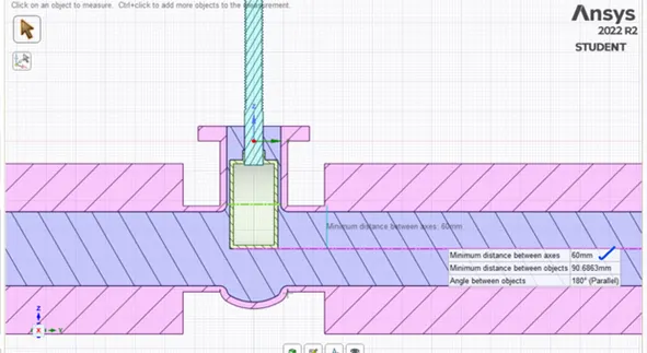
- Cross sectional view of the gate valve with fluid volume.
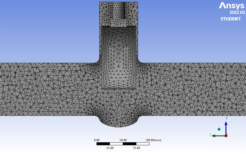
- Cross sectional view of the mesh elements for the fluid volume.
|
Cells |
Faces |
Nodes |
|
217210 |
449059 |
43784 |
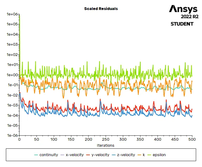
RESIDUALS PLOT :-
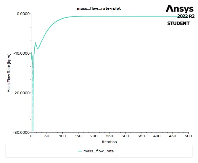
MASS FLOW RATE AT OUTLET - PLOT :-
Solution status :-
- From the above plots, we see that the solution got converged at 250th iteration since the rate at which residuals and mass flow rate at oulet value changes become constant over iteration.
|
Value |
Absolute Criteria |
Convergence Status |
|
|
continuity |
0.03571703 |
0.001 |
Not Converged |
|
x-velocity |
0.0001077264 |
0.001 |
Converged |
|
y-velocity |
0.0004059597 |
0.001 |
Converged |
|
z-velocity |
0.0001022925 |
0.001 |
Converged |
|
k |
0.1995665 |
0.001 |
Not Converged |
|
epsilon |
0.8470737 |
0.001 |
Not Converged |
Report definitions :-
|
mass_flow_rate |
-0.6296555 |
kg/s |
Calculation of Volumetric flow rate :-
We know that,
Volume flow rate (Q) = Mass flow rate / Density of the fluid (water)
Q = 0.6296555/998.2
|
Volumetric Flow Rate |
-0.0006307909 |
m^3/s |
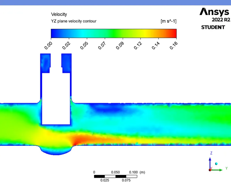
VELOCITY CONTOUR :-
-
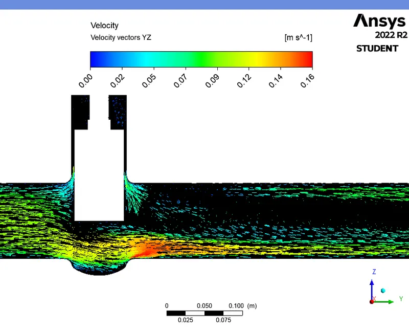
VELOCITY VECTORS :-
CASE 7 (Gate valve lift - 70mm) :-
- Create another design point in the Parameter set- window for lift value of 70mm and update the design point.
PRE-PROCESSING :-
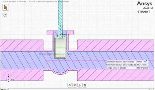
- Cross sectional view of the gate valve with fluid volume.
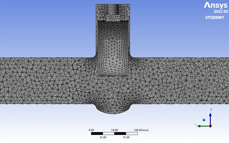
- Cross sectional view of the mesh elements for the fluid volume.
|
Cells |
Faces |
Nodes |
|
216311 |
447186 |
43598 |
RESIDUALS PLOT :-
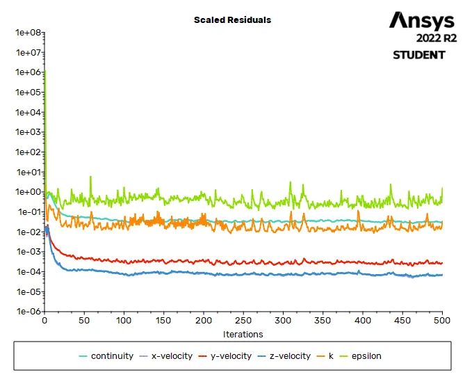
MASS FLOW RATE AT OUTLET - PLOT :-
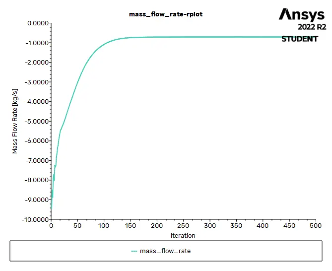
Solution status :-
- From the above plots, we see that the solution got converged at 450th iteration since the rate at which residuals and mass flow rate at oulet value changes become constant over iteration.
|
Value |
Absolute Criteria |
Convergence Status |
|
|
continuity |
0.03242812 |
0.001 |
Not Converged |
|
x-velocity |
6.798382e-05 |
0.001 |
Converged |
|
y-velocity |
0.000274682 |
0.001 |
Converged |
|
z-velocity |
7.156774e-05 |
0.001 |
Converged |
|
k |
0.03291835 |
0.001 |
Not Converged |
|
epsilon |
1.557364 |
0.001 |
Not Converged |
Report definitions :-
|
mass_flow_rate |
-0.7082934 |
kg/s |
Calculation of Volumetric flow rate :-
We know that,
Volume flow rate (Q) = Mass flow rate / Density of the fluid (water)
Q = 0.7082934/998.2
|
Volumetric Flow Rate |
-0.0007095706 |
m^3/s |
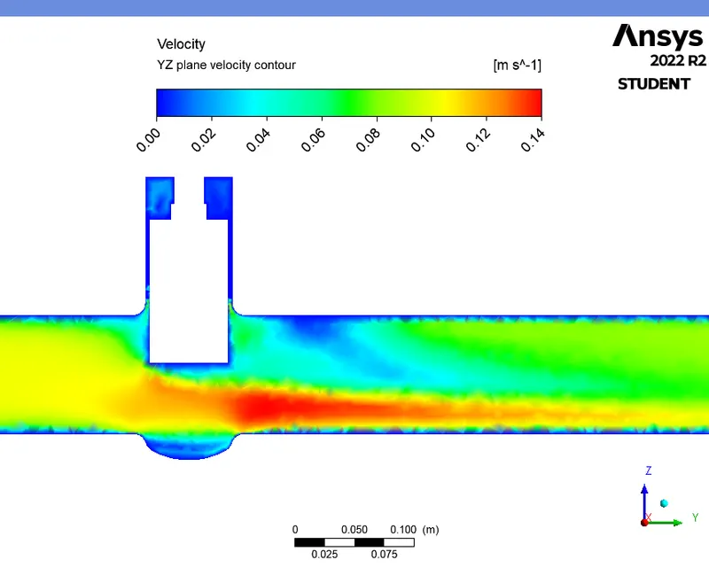
VELOCITY CONTOUR :-
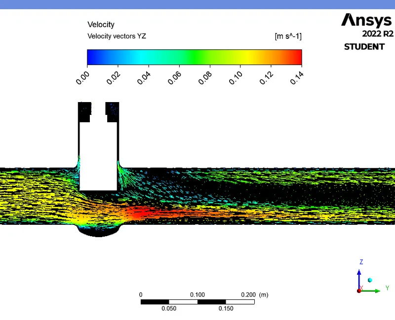
VELOCITY VECTORS :-
CASE 8 (Gate valve lift - 80mm) :-
- Create another design point in the Parameter set window for lift value of 80mm and update the design point.
PRE-PROCESSING :-
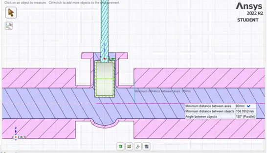
- Cross sectional view of the gate valve with fluid volume.
- Cross sectional view of the mesh elements for the fluid volume.
|
Cells |
Faces |
Nodes |
|
214982 |
444437 |
43339 |
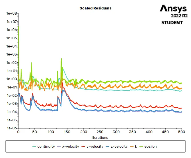
RESIDUALS PLOT :-
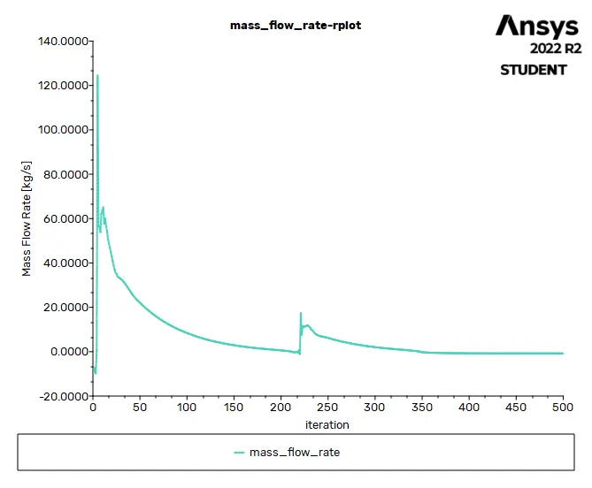
MASS FLOW RATE AT OUTLET - PLOT :-
Solution status :-
- From the above plots, we see that the solution got converged at 450th iteration since the rate at which residuals and mass flow rate at oulet value changes become constant over iteration.
|
Value |
Absolute Criteria |
Convergence Status |
|
|
continuity |
0.03739197 |
0.001 |
Not Converged |
|
x-velocity |
8.598935e-05 |
0.001 |
Converged |
|
y-velocity |
0.0002903818 |
0.001 |
Converged |
|
z-velocity |
0.0001033664 |
0.001 |
Converged |
|
k |
0.06905487 |
0.001 |
Not Converged |
|
epsilon |
0.3593759 |
0.001 |
Not Converged |
Report definitions :-
|
mass_flow_rate |
-0.7851822 |
kg/s |
Calculation of Volumetric flow rate :-
We know that,
Volume flow rate (Q) = Mass flow rate / Density of the fluid (water)
Q = 0.7851822/998.2
|
Volumetric Flow Rate |
-0.00078659807 |
m^3/s |
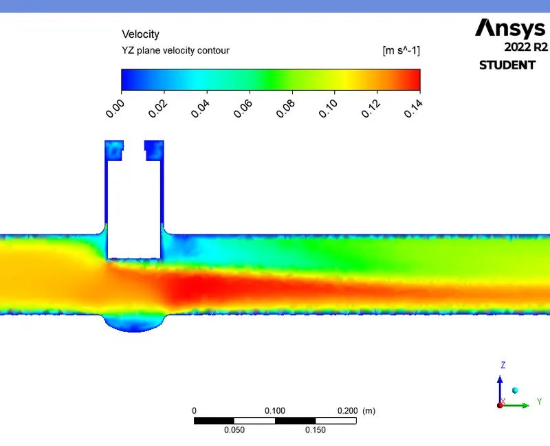
VELOCITY CONTOUR :-
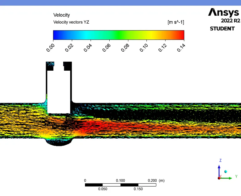
VELOCITY VECTORS :-
Parameter set window :
|
|
GATE VALVE POSITION (in 'mm') |
NUMBER OF MESH ELEMENTS |
MASS FLOW RATE AT OUTLET (in 'kg/s') |
VOLUMETRIC FLOW RATE (Q) |
GAUGE PRESSURE DIFFERENCE ACROSS THE VALVE (in 'bar') |
FLOW FACTOR (KV)(KV) |
FLOW COEFFICIENT (CV)(CV) |
|
|
(in 'm^3/s') |
(in 'm^3/hr') |
|||||||
|
CASE - 1 |
10 |
226230 |
0.1426206 |
0.00014287778 |
0.51436 |
0.0001 |
51.436 |
59.4636 |
|
CASE - 2 |
20 |
224561 |
0.2293705 |
0.000229784 |
0.8272224 |
0.0001 |
82.722 |
95.6326 |
|
CASE - 3 |
30 |
222083 |
0.3468929 |
0.0003475184 |
1.251066 |
0.0001 |
125.1066 |
144.632 |
|
CASE - 4 |
40 |
219283 |
0.4503665 |
0.0004511786 |
1.624243 |
0.0001 |
162.4243 |
187.774 |
|
CASE - 5 |
50 |
218410 |
0.5353329 |
0.000536298 |
1.930673 |
0.0001 |
193.0673 |
223.199 |
|
CASE - 6 |
60 |
217210 |
0.6296555 |
0.0006307909 |
2.270847 |
0.0001 |
227.0847 |
262.5257 |
|
CASE - 7 |
70 |
216311 |
0.7082934 |
0.0007095706 |
2.55445 |
0.0001 |
255.445 |
295.312 |
|
CASE - 8 |
80 |
214982 |
0.7851822 |
0.00078659807 |
2.83175 |
0.0001 |
283.175 |
327.37 |
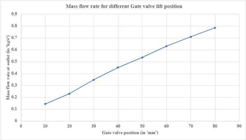
Mass flow rate for different valve position :
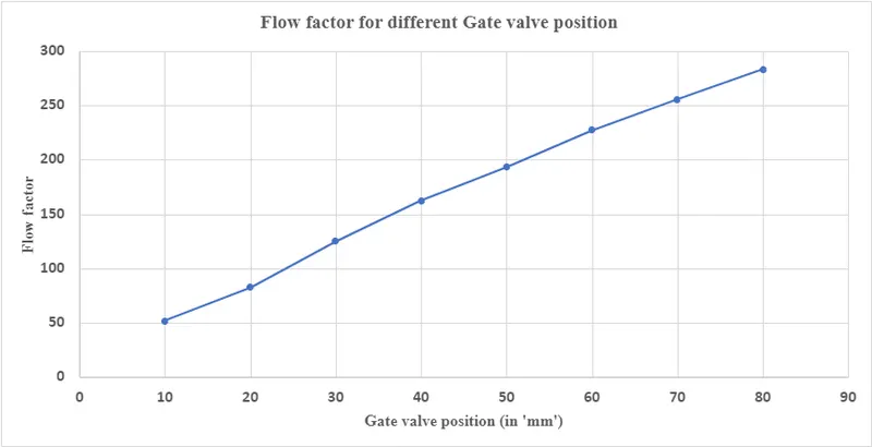
Flow factor for different valve position :
CONCLUSION:-
- Mass flow rate gradually increases as the lift of gate disc is increased.
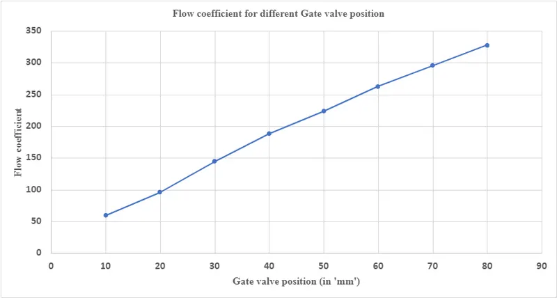
- The variation of flow coefficient and flow factor with the opening of the valve is studied by using parametric method.
- Parametric study is time reducing option when studying the effects of changes of certain parameters of a system.
- Flow coefficient plays an important role in the selection of valve and sizing of a valve, so calculating it is necessary.
- Flow coefficient also helps in computing the efficiency of the system and the effectt of pressure on the system.