Parametric study on Gate valve simulation

A gate valve is generally used to completely shut off fluid flow or, in the fully open position, provide full flow in a pipeline. Thus it is used either in fully closed or fully open positions. A gate valve consists of a valve body, seat and disc, a spindle, gland, and a wheel for operating the valve. The seat and the gate together perform the function of shutting off the flow of fluid. A typical gate valve is shown in Figure 12.9.

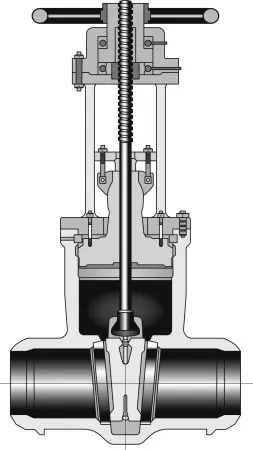
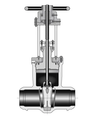
Gate valves are generally not suitable for regulating flow or pressure or operating in a partially open condition. For this service, a plug valve or a control valve should be used. It must be noted that because of the type of construction a gate valve requires many turns of the handwheel to completely open or close the valve. When fully opened, gate valves offer little resistance to flow, and its equivalent length to diameter ratio (L/D) is approximately 8.

The gate valves used in the mainlines carrying oil or gas must be of the full bore or through conduit design to enable smooth passage of scrapers or pigs used for cleaning or monitoring pipelines. Such gate valves are referred to as full bore or through conduit gate valves.

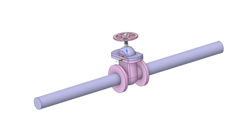
Now here we going to perform a simulation on the gate valve for which we have the STEP file. Here we going to lift the gate disc inside the valve which will vary from 10% to 80% of the total open conditions.

First, we gonna drag and drop the STEP file for the Gate valve in the SpaceClaim.

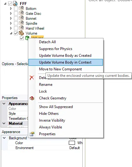
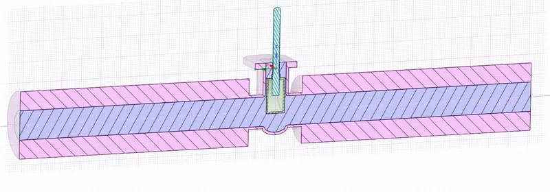
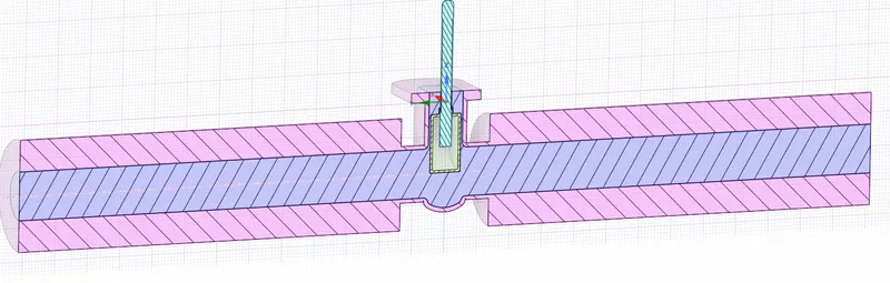
and extend the Inlet and Outlet by 800m and extract it with VOLUME EXTRACT.

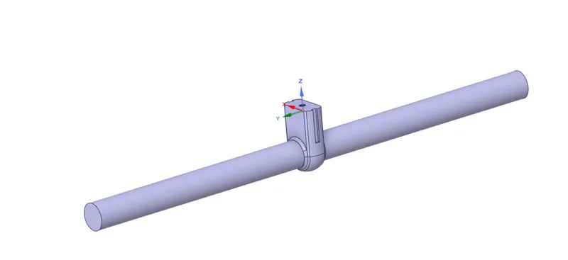
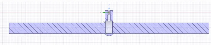
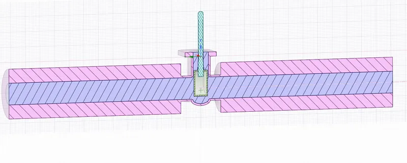
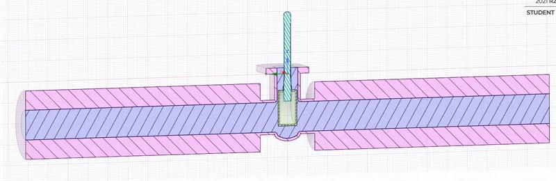
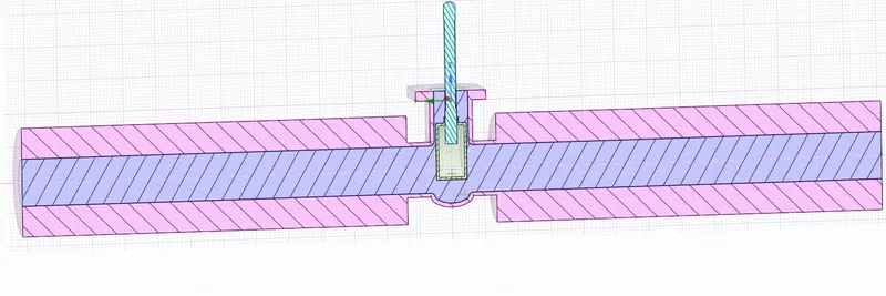
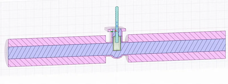
Now first we are going to try for 10% of the opening and then we go further til 80%. This is what the opening of the gate valve at 10% looks like.

Now we are going to for Mesh part in meshing.

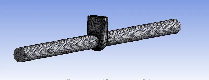
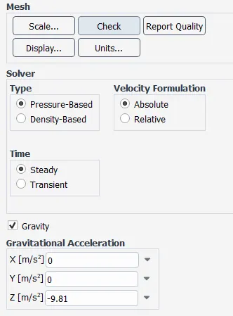
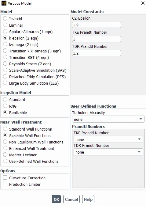
When the meshing is done we go to fluent and add viscous model and set up the case for simulation.

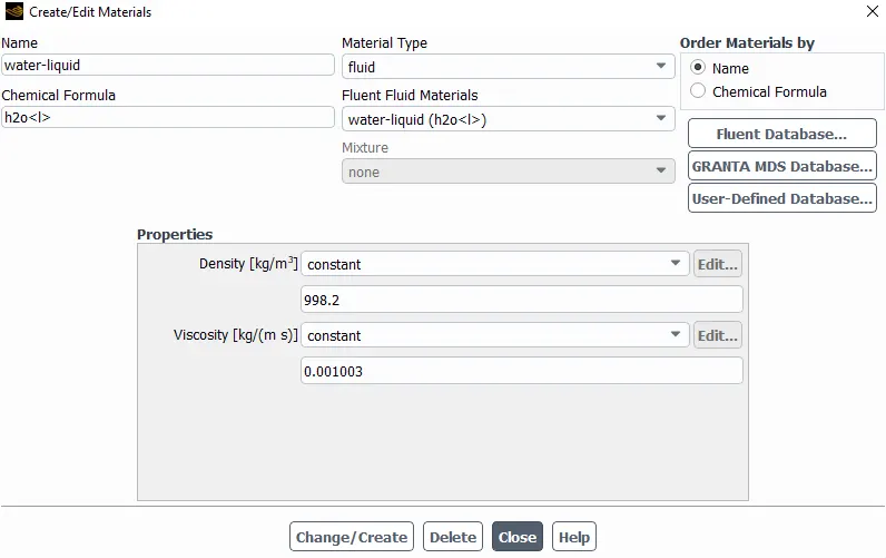
Here we create new materials to add in the cell zones for the simulation.

and then we edit the boundary conditions.

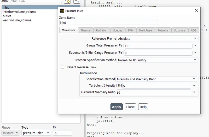
and then we ADD water and DELETE air in the cell zones.

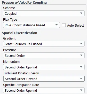
for methods we preferred COUPLED with first-order upwind only if we face issues on mass-flow excitation. or else we are good to go with second-order upwind.

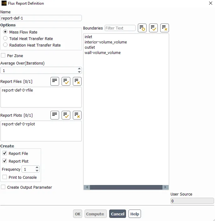
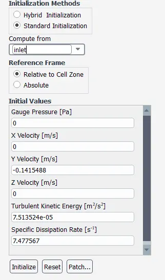
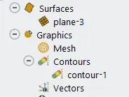
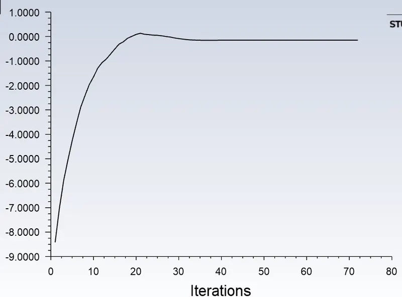
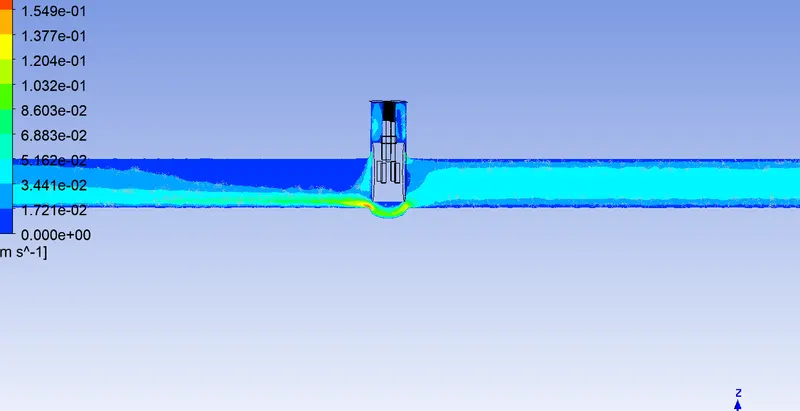
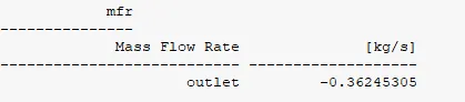
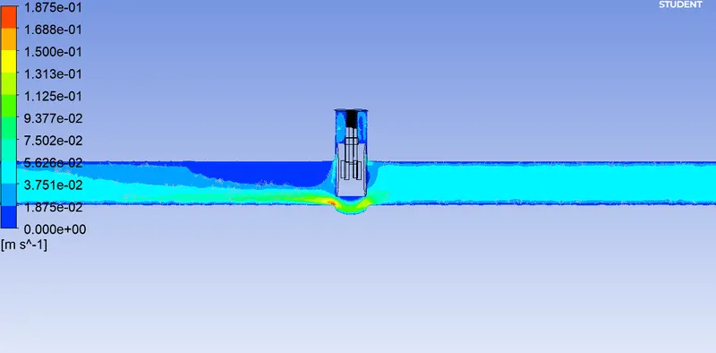
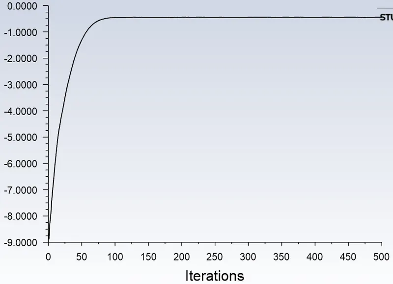
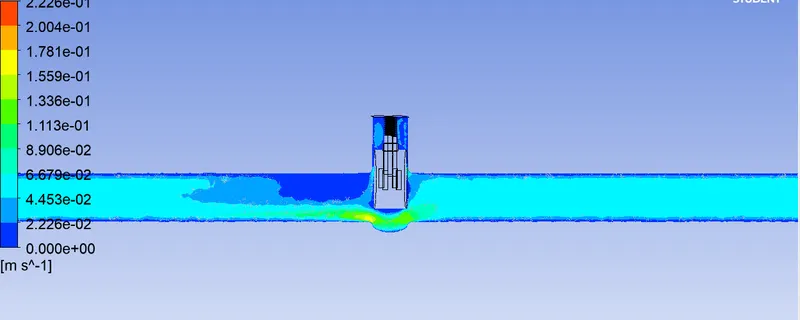
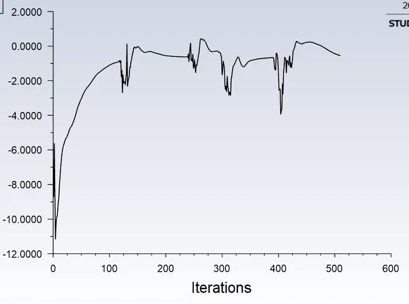
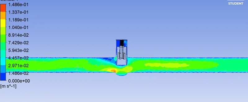
Now we have added a flux definition report where we determine the mass flow rate of the channel. And we initialize the setup, computing from INLET. Also by adding the contour plot on a separate plane.

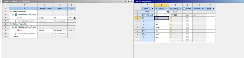
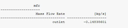
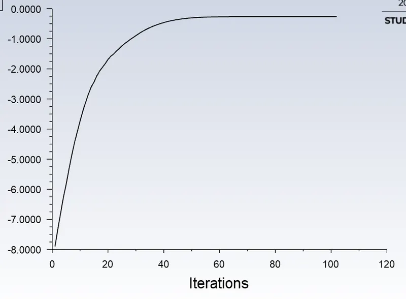
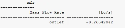
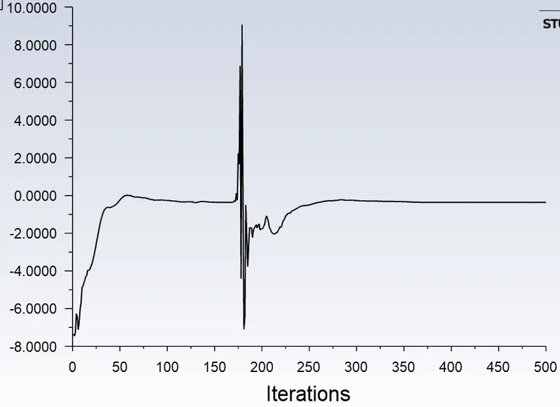
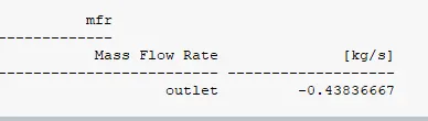
Now we run the simulation here and notice the mass flow rate at the end of the report. And right after that, we are going to add more parametric values on a separate section in the space claim.

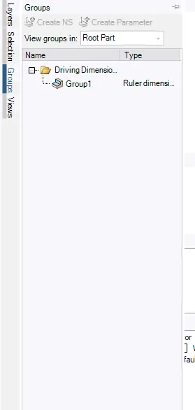
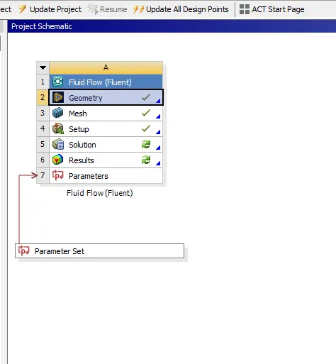
and in the Home window of the workbench, you can see the new added bottom section.

OUTPUT:

1. Obtain the mass flow rates at the outlet for each design point.

we consider that the lift can happen til 75mm and that every small percentage of what it chan represent as lift variation.

1. Lift at 10% at 7.5mm

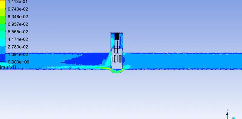
2. Lift at 20% at 15mm

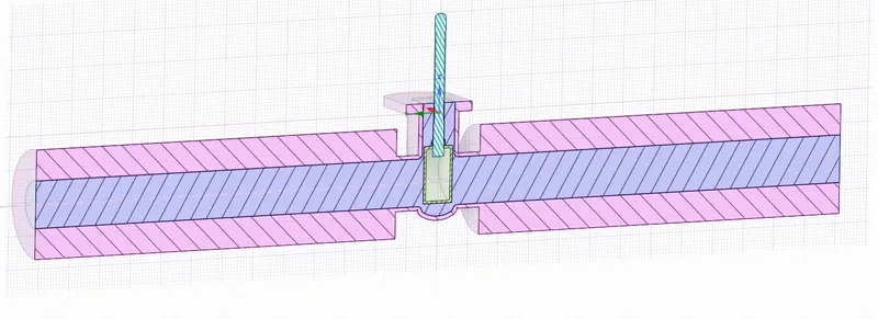
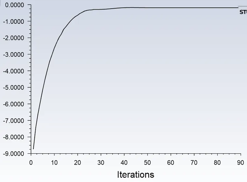
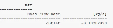
3. Lift at 30% at 22.5mm

4. Lift at 40% at 30mm

5. Lift at 50% at 37.5mm

6. Lift at 60% at 45mm

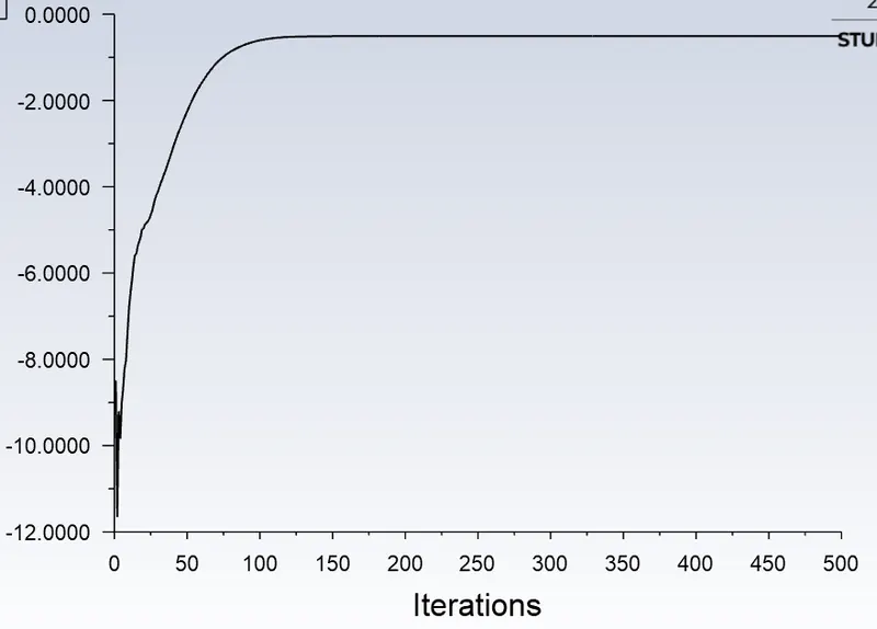
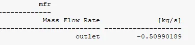
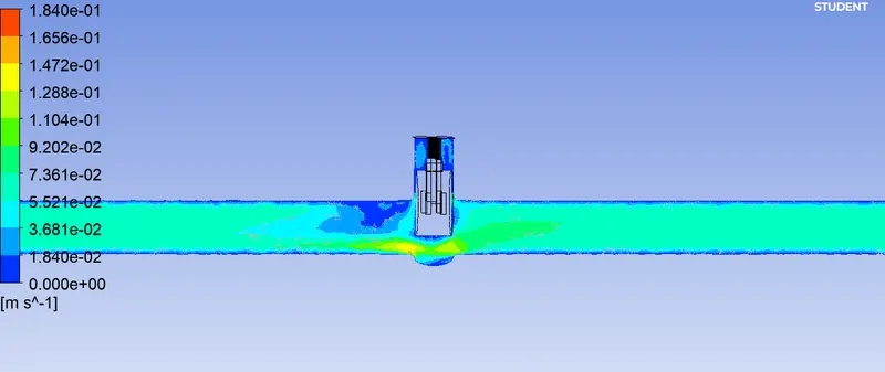
7. Lift at 70% at 52.5mm

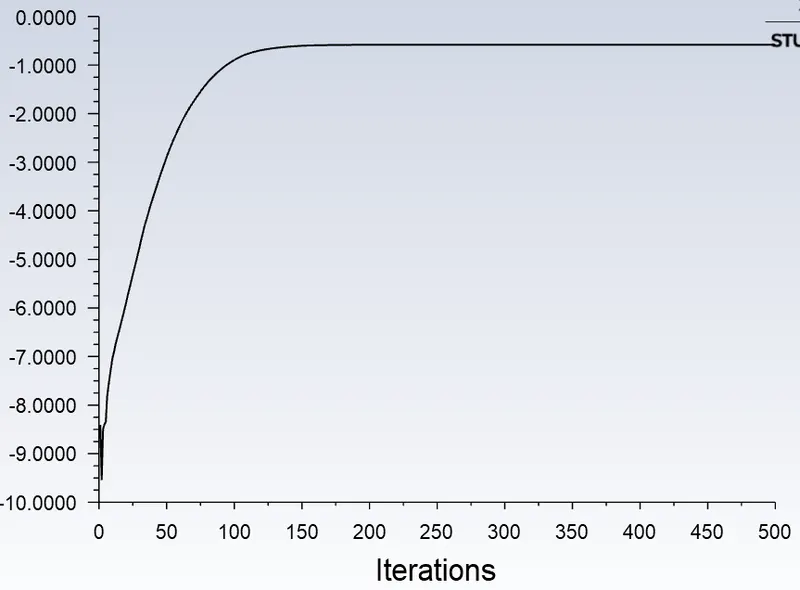
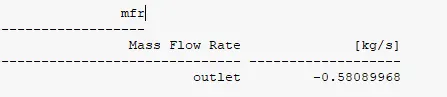
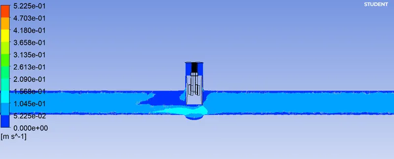
8. Lift at 80% at 60mm

2. Calculate the flow coefficient and flow factor for each opening and plot the graph.

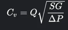is flow coefficient

K_v = 0.862 C_v is flow factor

1. Gate Lift at 7.5mm at 10%

Q = 0.14, SG of water = 1, ΔP = 10

Flow coefficient = 0.04427

Flow factor = 0.862 x 0.04427 = 0.381

2. Gate Lift at 15 mm at 20%

Q = 0.187, SG of water = 1, ΔP = 10

Flow coefficient = 0.05913

Flow factor = 0.862 x 0.05913 = 0.0509

3. Gate Lift at 22.5mm at 30%

Q = 0.265, SG of water = 1, ΔP = 10

Flow coefficient = 0.0838

Flow factor = 0.862 x 0.4427 = 0.0722

4. Gate Lift at 30mm at 40%

Q = 0.362, SG of water = 1, ΔP = 10

Flow coefficient = 0.1144

Flow factor = 0.862 x 0.1144 = 0.098

5. Gate Lift at 37.5mm at 50%

Q = 0.44, SG of water = 1, ΔP = 10

Flow coefficient = 0.1391

Flow factor = 0.862 x 0.4427 = 0.1199

6. Gate Lift at 45mm at 60%

Q = 0.509, SG of water = 1, ΔP = 10

Flow coefficient = 0.1609

Flow factor = 0.862 x 0.1609 = 0.1387

7. Gate Lift at 52.5mm at 70%

Q = 0.5808, SG of water = 1, ΔP = 10

Flow coefficient = 0.1836

Flow factor = 0.862 x 0.1836 = 0.1583

8. Gate Lift at 60 mm at 80%

Q = 0.4383, SG of water = 1, ΔP = 10

Flow coefficient = 0.1386

Flow factor = 0.862 x 0.1386 = 0.1194

3. Discuss the results of the mass flow rate and flow coefficient.

The flow coefficient ϕ is a measure of the angle of incidence of the flow and the aaerodynamic forces developed are critically dependent upon this parameter. Typical results based on predictions and experiments of the non-dimensional pressure drop p*=Δp/(ρω2Dt2)">p*=Δp/(ρω2Dt2) and efficiency are shown in Figures. For a wells turbine a linear relationship exists between pressure drop and the flow rate [Figure 9.26(a)] and this fact can be employed when making a match between a turbine and anoscillating water column that also has a similar characteristic.

In a high flow high inlet eye diameter 3D impeller, the blade angles along the leading edge may be varied from disk to shroud to match the incoming flow field and obtain optimum incidence angles. This typically occurs at the impeller’sdesign flow arte, and any increase or decreasein flow rate will result in nonoptimal incidence and lower performance. The efficiency of an impeller is a function of the inlet flow coefficient. As the flow coefficient increases, there is an increase in impeller efficiency. While it would seem that only 3D impellers should be used due to their higher efficiency, it generally results in a larger stage spacing (axial length), which could increase rotordynamic complexity and cost. Consequently 3D impellers are typically used only for the first or first few impellers unless an incoming sidestream calls for a high flow coefficient stage further down the machine. High flow and high-efficiency design staging may require reduced speeds due to higher stress levels encountered. The compressor supplier’s and designer’s experience in selecting various flow coefficient impellers should be carefully reviewed.

The influencing characteristic of cross-flow coefficient between fracture and matrix in the streamline numerical well testing interpretation model for a multi-layer reservoir in dual-porosity media is still studied based on the typical model above.

References:

Gate Valve - an overview | ScienceDirect Topics

Flow Coefficient - an overview | ScienceDirect Topics

Flow Coefficient C_v vs. Flow Factor K_v (engineeringtoolbox.com)