Week - 9 Material Modeling from Raw Data

Aim:

By using the diagram of true stress strain curve given data curve by using get data graph digitizer.Crete a material 024 for an Dogbone specimen.Finially validate the mat card by performing the tensile test on Dogbone specimen and compare the results.

Objective:

1. Extract the data from the diagram
2. Clean the data and visually confirm that it matches the original data and the elastic modulus is 20.9E+06 psi.
3. Convert the data to (kg-mm-ms) unit system
4. Process the data and create the material as demonstrated
5. Use the material model with a dogbone specimen and validate the same..

Procedure:

Data Extraction from the curve image:

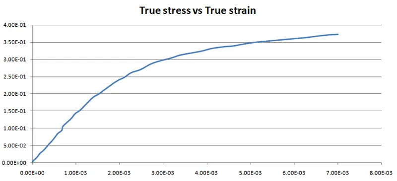
In this case ,we got an image representing a True stress vs true strain with three different strain rate, From the graph, we can see the material behavior with elastic and plastic region .The models at MAT_24 = MAT_PIECEWISE_LINEAR_PLASTICITY.

First of all the image available in png format ,but this format won’t supports ,so we have to convert into jpg format.After that we provide the xmin,xmax,ymin and ymax valve and select no of point on curve and export to excel.

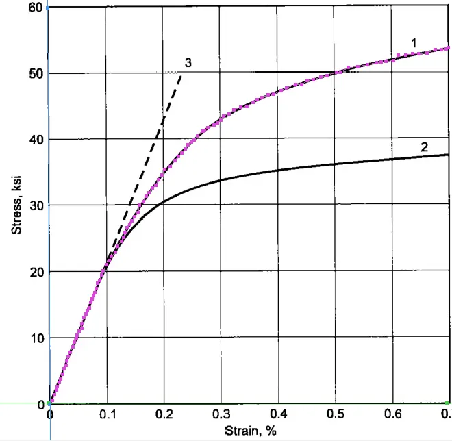
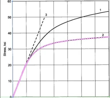
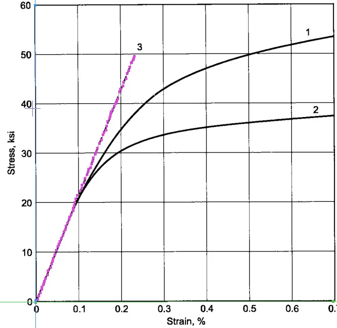
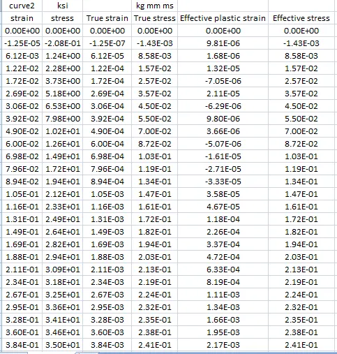
Data calculation stress-strain curve

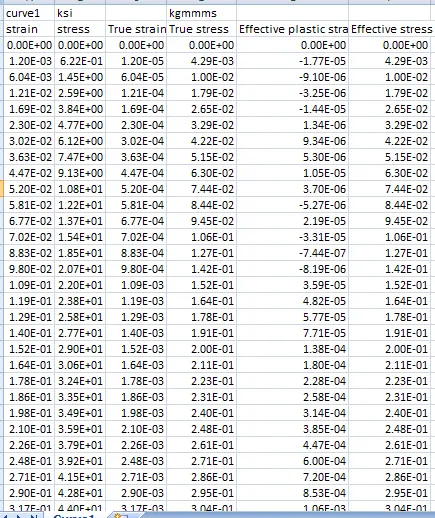
The number of stress-strain points generated and exports to Microsoft excel.

The material card model we use SI units is kg/mm/ms ,but stress and strain graph is Ksi for stress and percentage for strain resp.

1Ksi = 6894.76 x 10^3 kg/m x s^2

1Ksi = 6.895 x 10^-3 kg/mm*ms

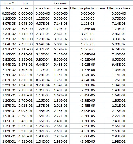
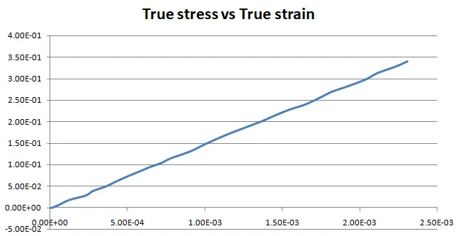
True strain = ln (1+ engineer strain)

True stress= Engineer stress x(1+Engineer strain)

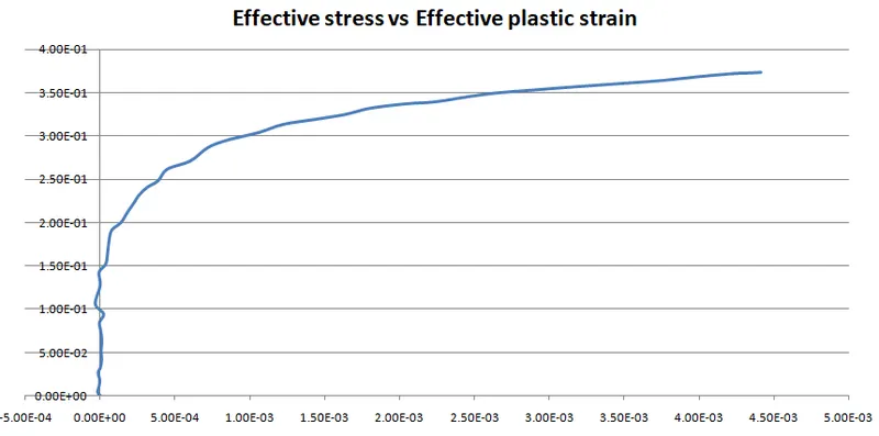
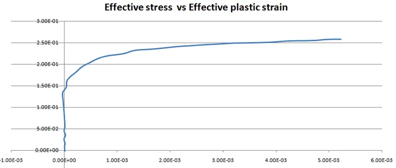
Effective Plastic strain = true strain - true stress / E

where , elastic modulus is 20.9E+06 psi. In our unit should be in kg mm ms

20.9E+06 psi = 144100.4 x 10^-3

=144.1004

curve 1

curve 2

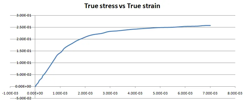
Curve3

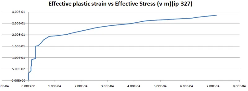
By using the curve 1 elastic plastic strain vs effective stress plot the data of the curve to mat 024 card

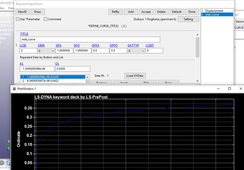
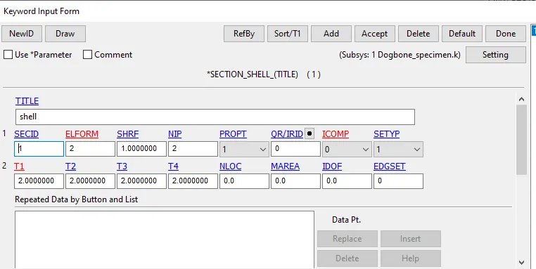
Assign material property and shell section MAT_024 import curve 1 that mentioned above.

.

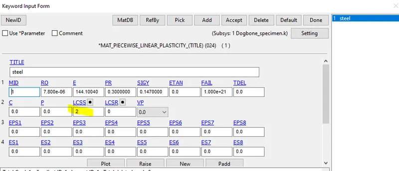
Boundary condition

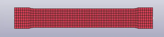
Since we have tensile test where one end of the specimen is fixed and the displacement is added to the end of the specimen ,so we will use two bcs for these specimen

To fix one end of the specimen as test procedure we constraint all dof expect y direction

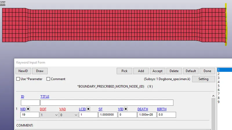
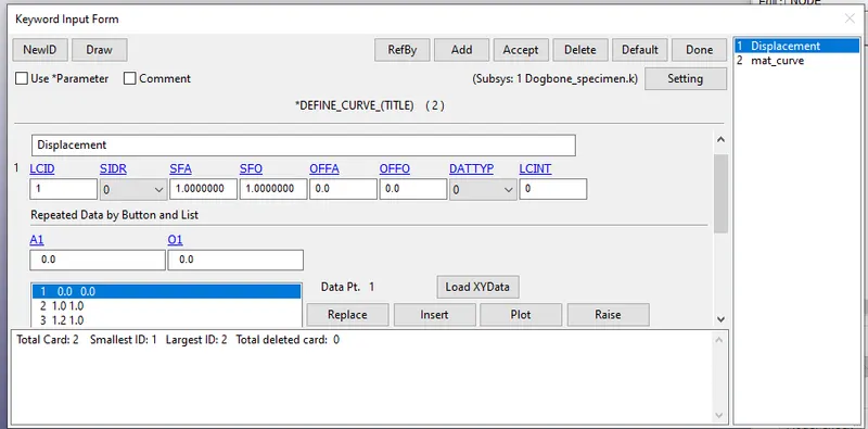
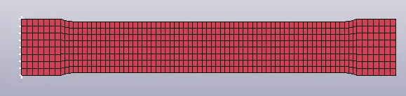
We will select the mid node on edge of the both end of the specimen

Control cards

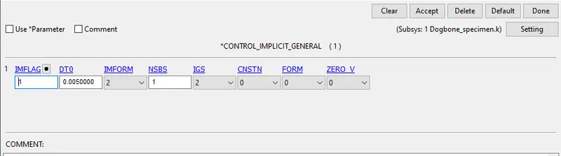
(CONTROL_IMPLICIT_GENERAL

It activates Implicit analysis and define control parameters

IMFLG – Implicit/Explicit analysis type flag1- Implicit analysis

DTO- Intial time steps size for implicit analysis 0.005

IMFORM – Element formulation flag for seamless spring back : 2 retain original elements

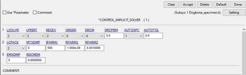
*CONTROL_IMPLICIT_SOLUTION

NSOLVER – Solution method for implicit analysis 12 for Non Linear problem

ILIMIT – Iteration limit between automatic st

MAXREF Stiffness reformation limit per time step.15

DCTOL Displacement relative convergence tolerance 001

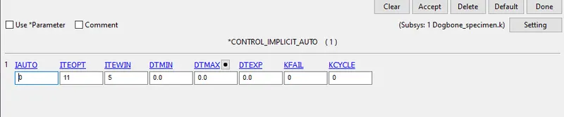
*CONTROL_IMPLICIT_AUTO

IAUTO set automatically adjust time step size

ITEOPT Optimum equilibrium iteration count per time step 11

ITEWIN Allowable iteration window 5

DTMIN Minimum allowable time step size.

DTMAX Maximum allowable time step size.

Database cretion

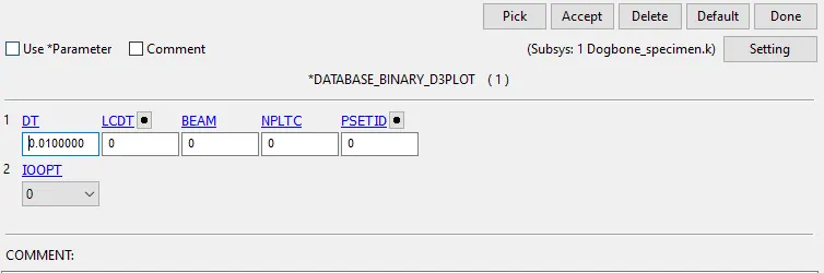
*BINARY_D3PLOT – It defines thefrequency of animation files is set to be 0.010ms

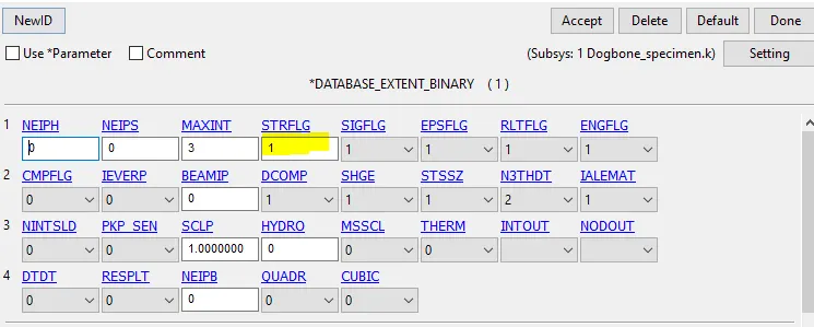
*DATABASE_EXTEND_BINARY, this writes the strain tensor STRFLG is set to 1.

ASCII formats

GLSTAT – global data

MATSUM – material energies

ELOUT – element output data

Results:

Conculsion

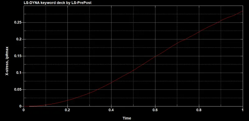
The stress strain is extracted and validated from the images using a data digitizer by MAT_024 – PIECEWISE LINEAR PLASTICITY, Which captures the actual stress-strain behavior similarly.