Material Modeling from Raw Data using LS-DYNA

Objective:

By Using the diagram of the true stress-strain curve given for graphite iron casting, create a material model for the Dogbone specimen. Validate the created material model card by performing a tensile test on a Dogbone specimen. Finally, the results are compared.

Procedure for material modeling:

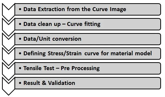
Data Extraction from the Curve Image:

In general, The material test data is collected as

Force vs Displacement

Engineering stress vs strain

Raw data

The image representing the curve of the data points.

In this case, We got an Image representing a True Stress/ Strain curve with 3 different strain rate, From the graph, we can see The material shows elasto-plastic behavior with the elastic and plastic region Although many material models exist for elasto-plastic, one of the most robust models is *MAT_024 or *MAT_PIECEWISE_LINEAR_PLASTICITY. This material model is the standard workhorse and is the recommended starting point for elastic-plastic simulation of metals and general plastics since it can also handle viscoelastic behavior (i.e., strain-rate dependency).

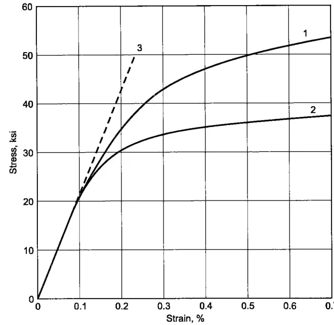
From the above Plot, we will take The curve 2 data point for our material modeling purpose. By using the GETDATA GRAPH DIGITIZER application, the data points are extracted from an image file.

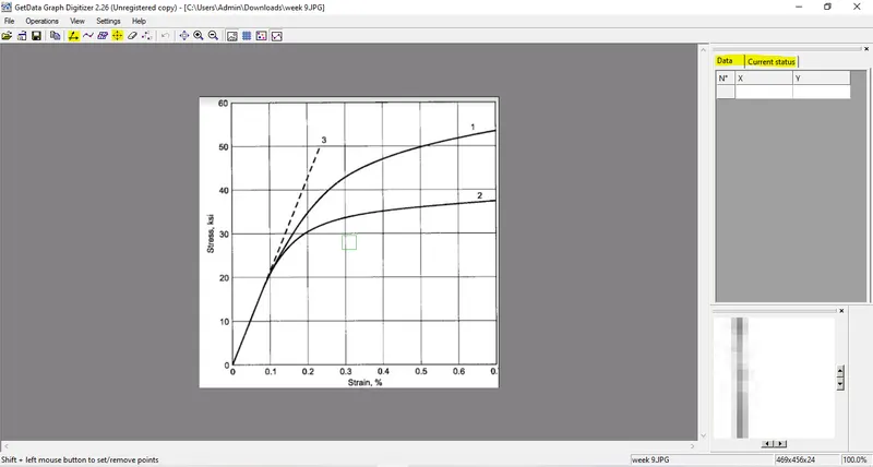
First, the image is processed and the x-scale and y-scale are decided(min, max values). Then the data points are selected from the image. Selected data points are displayed with the X and Y coordinates in the top right corner of the application. Finally, the file is saved in a suitable format in the local directory file.

Data clean up–Curve fitting:

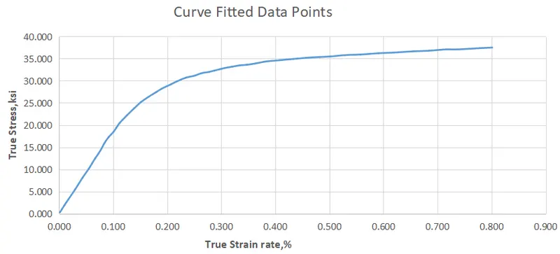
The data point extracted from the image is always noisy and the data points are selected manually by picking each point so they will be some human error and Since, Ls-Dyna will accept only the monotonically increasing curves. We need to clean up the curve and fit the rough data. This is done using Microsoft EXCEL.

Data/Unit conversion:

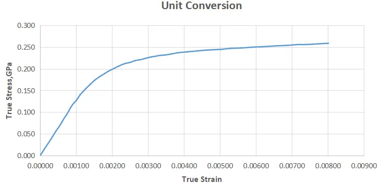
For the Material card model we are using the SI unit i.e Kg/mm/ms but if we noticed from the Stress and Strain graph units is give in ksi for Stress and percentage for Strain respectively. So the unit of stress has to be changed from ksi to GPa and Strain has to change from percentage to actual value.

0.2% offset Yield Strength:

The conversion from elasticity to plasticity can be very subtle for many materials. So it might not be always very easy to figure out the yield point, that is the point on the stress-strain curve, where elasticity changes to plasticity. In other words, at the yield point, if you let go of the deforming force, the material will not come back to its original form there will be some amount of permanent deformation.

In this case, the offset yield strength is determined. A line is constructed parallel to the initial portion of the stress-strain curve but offset by 0.002 in/in (0.2%) from the origin. The 0.2% offset yield strength is the stress at which the constructed line intersects the stress-strain curve as shown:

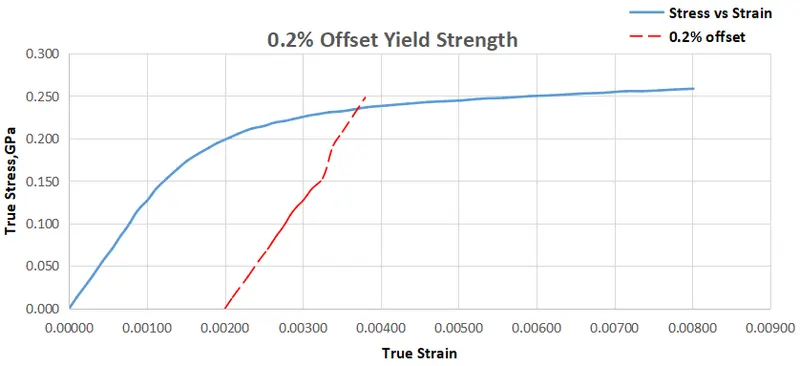
0.2% offset yield strength : 0.248211GPa.

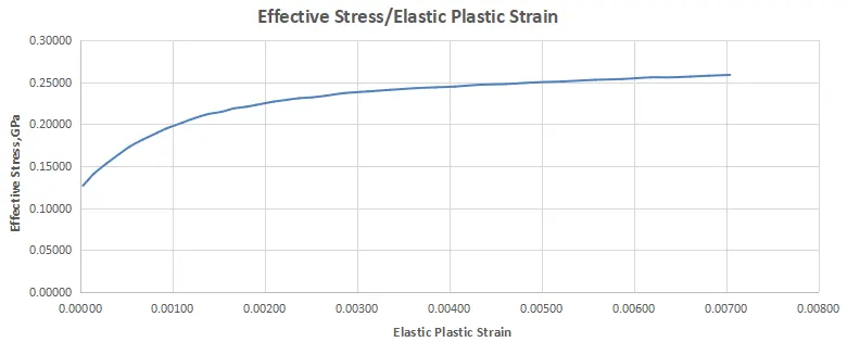
Once the unit conversion is done, we can see the extracted data are True stress and True strain But to define a Stress-Strain curve in *MAT_24 card, We have to define it in Effective stress and Effective plastic strain format. The true stress and strain values are converted into Effective stress and Effective plastic strain value using the following formula.

Effective stress = True stress

Effective plastic strain = True strain - True stress / E

Young’s Modulus is given for the material as 20E+6psi i.e 137.917GPa.

As the stress value increases, the recoverable strain (true stress/E) increases as well. For metals, E is very large compared to the yield stress so it's fairly common practice in the case of metals to just subtract off a constant value equal to the strain at initial yield from all subsequent strain values.

The True stress, in this case, is taken as the yield strength point from the true stress-strain curve. The value is about

True Stress / E = 0.13373/137.917

True Stress/E=0.00097.

The hardening curve which is defined in the material card should start ideally with yield strength and effective plastic strain (at yield strength) as a first point. So, we can remove the elastic region data point from the curve.

Importing the Model:

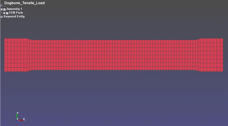
The model given for the Tensile load test is the Dogbone specimen. The command used to import the model is File menu--->open--->LS-DYNA Keyword file. The simple way to open the model is to press the shortcut key Ctrl+k.

Defining Stress/Strain curve for material model:

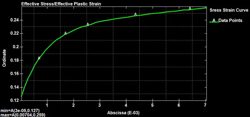
The stress/strain for the material is now in the form of Effective stress and Effective plastic strain which can be implemented on the *MAT_24 material card. These data points for the Stress/Strain curve are inserted *DEFINE_CURVE Card with LCID. The command used to define the curve is

Model--->Keyword Manager--->Define--->Curve.

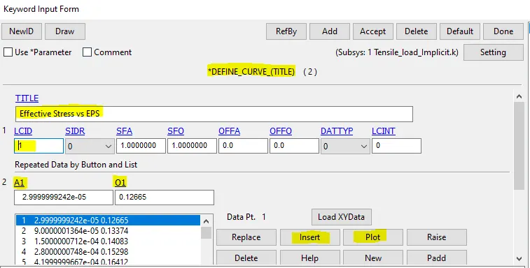
There are 38 data points are inserted into the curve.

Material Model:

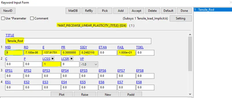
We will use graphite iron casting Properties for defining the material card.

1. MID: Material identification. A unique number or label not exceeding 8 Characters must be specified
2. RHO: Mass density= 7.100e-06
3. E: Young’s modulus = 144.10001 GPa
4. PR: Poisson’s ratio = 0.3
5. SIGY: Yield stress = 0.2293570 from 0.2% offset yield strength
6. LCSS: Load curve ID defining effective stress versus effective plastic strain.LCID from Define_curve

Creating Section card:

Since the imported model is Shell property, a shell section card is created with a thickness of 1mm. The command used for creating the section is Model--->Section--->Shell.

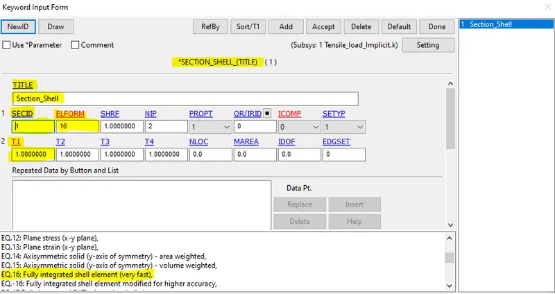
The ELFORM is selected as 16 means Fully Integrated Shell element formulation. The section card and the Material card are inserted into the dogbone specimen.

Boundary Condition:

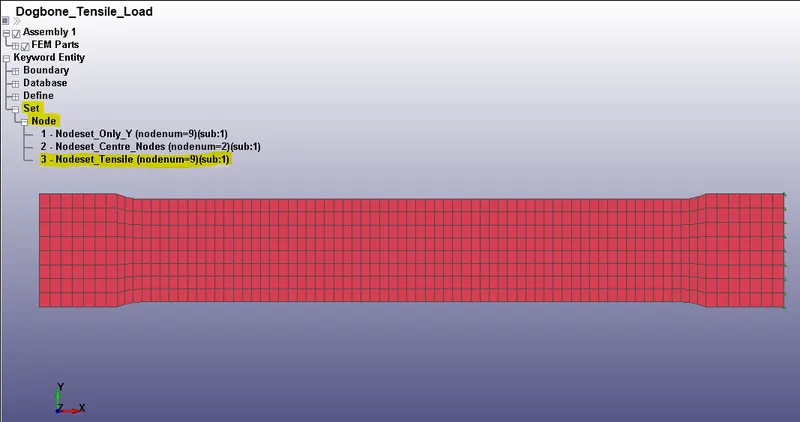
Since we performing a Tensile Test where one end of the specimen is fixed and the displacement is added to the other end so we will use two types of boundary conditions on the Specimen.

BOUNDARY_SPC_SET:

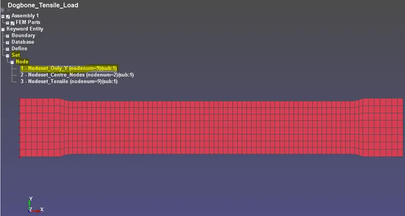
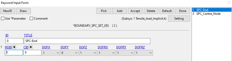
To fix one end of the specimen as a test procedure we will constraint all the DOF except Y direction (because specimen will elongate in the X direction and simultaneously contract in Y) for edge node on one end of the specimen.

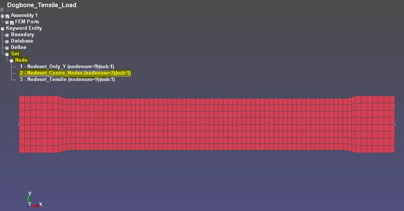
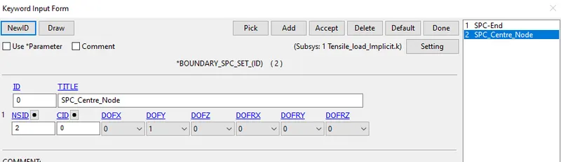
We will select the mid-node on edge of both ends of the specimen and constrain only the Y direction.

BOUNDARY_PRESCRIBED_MOTION_SET:

A set of nodes is created on the edge of the specimen in which displacement is applied.

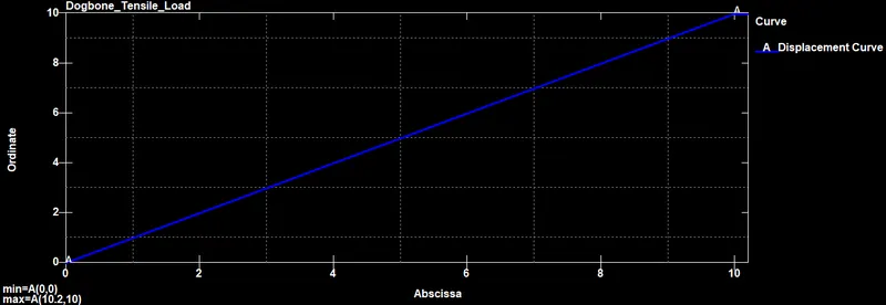
Displacement curve is created using Define_curve Card.

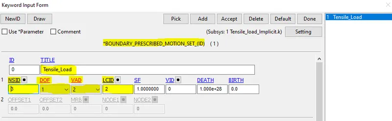
DOF in BOUNDARY_PRESCRIBED_MOTION_SET is set to be 1 which means displacement takes place in the X direction and VAD is set as 2 Displacement flag.

Control cards:

*CONTROL_IMPLICIT_GENERAL:

It activates Implicit analysis and defines associated control parameters. This keyword is required for all implicit analysis

• IMFLAG - Implicit/Explicit analysis type flag: 1- Implicit analysis.
• DT0 – Initial time step size for implicit analysis: 0.0050000.
• IMFORM - Element formulation flag for seamless spring back: 2 retain original element. formulation (default).

*CONTROL_IMPLICIT_SOLUTION:

The main use of these cards to specify whether a linear or nonlinear solution is desired.

• NSOLVER – Solution method for implicit analysis: 12 For Non-linear problem.
• ILIMIT-Iteration limit between automatic stiffness reformations: 11.
• MAXREF- Stiffness reformation limit per time step: 15.
• DCTOL- Displacement relative convergence tolerance: 001.
• DNORM- Displacement norm for convergence test: 2 (Increment as a function of total displacement).

*CONTROL_IMPLICIT_AUTO

This card has been defined to adjusts the time step size automatically.

• IAUTOset to 1 which automatically adjusts the timestep size.
• ITEOPToptimizes the operation count step:100.
• ITEWINis the iteration window: 50.
• DTMIN Minimum allowable time step size: 0.005.
• DTMAXMaximum allowable time step size:5.

Database Creation:

*BINARY_D3PLOT - It defines the frequency at which the animation file is to be created and is set to 5.000e-05 ms

*DATABASE_HISTORY_NODE defines nodes on Specimen to measure the Effective Stress and Plastic Strain in both shell and node which possess high deformation during the tensile load.

*DATABASE_EXTEND_BINARY, this writes the strain tensor to d3plot when STRFLG is set to 1.

ASCII_option keyword:

The output request in ASCII format, The following keyword are Activated,

1. GLSTAT- Global Data.
2. MATSUM- Material Energies and,
3. ELOUT- Element Output Data.

Results:

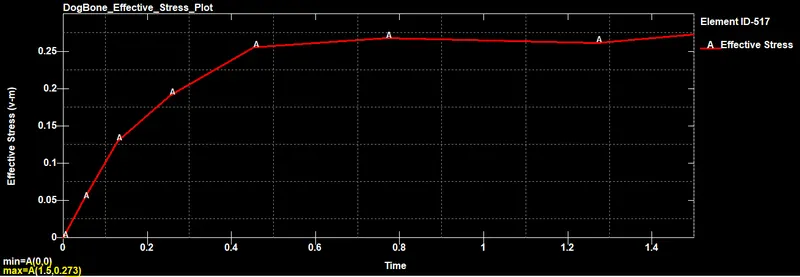
Effective Stress(Von-Mises Stress):

Max Stress: 0.272756GPa

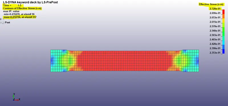
Effective Stress is plotted for the element-ID 517

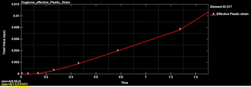
Effective Plastic Strain:

Max Effective Plastic Strain: 1.073E-02.

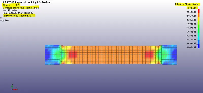
Effective Plastic Strain is plotted for element-ID 517.

Stress-strain Curve:

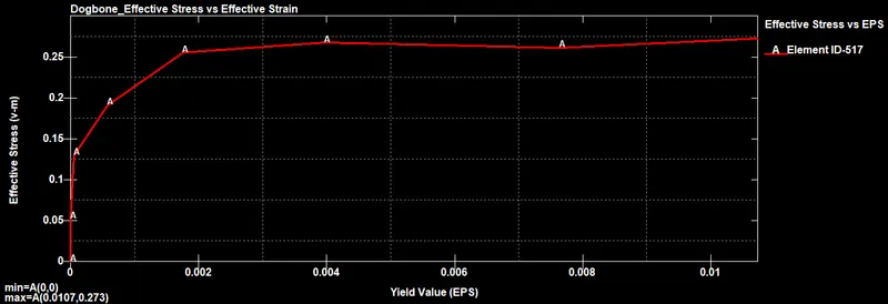
Comparison of results:

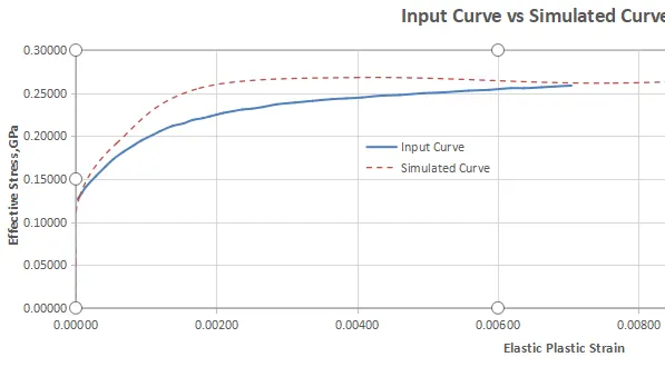
Material defined stress-strain data and simulated stress-strain data are compared. It can be seen that the elastic part is linear. The linear elastic part is calculated directly through the given young’s modulus and yielding starts after the first defined yield point in the hardening curve.

Conclusion :

The stress-strain data extracted from the image is validated with the MAT_024(Piecewise linear plasticity) material model. The stress-strain behavior after yielding is considered by a hardening curve which is given as an input through MAT_024 card.

The MAT_024 material model captures the actual stress-strain behavior in a similar manner and almost matched the defined stress-strain curve in the material model. Also, we saw little variation in the simulation data, which can due to the lack of information like density and Poisson’s ratio for the raw data, Mesh Size of the model, or defining proper strain rate.

This variation can be fine-tuned by trying different values of these properties and by selecting more data points to better capture the curve feature.