Material Modeling from Raw Data for linear plastic (MAT_024) material Using LS-Dyna

AIM: To model and validate an Elasto-Plastic material for a given stress-strain data Using LS-Dyna.

OBJECTIVE: Here is the workflow:

• Extract the data from the diagram
• Clean the data and visually confirm that it matches the original data and the elastic modulus is 20.9E+06 psi.
• Convert the data to (kg-mm-ms) unit system
• Process the data and create the material as demonstrated
• Use the material model with a dogbone specimen and validate the same.

ABSTRACT:

In this challenge, we are going to build the material model using the raw data extracted from a stress and strain plot. The diagram provided in the challenge is of the true stress-strain curve of graphite iron casting. For extracting data from the diagram we use a data digitizer tool. Then with this, we will define the curve(True stress vs Effective strain) for the material.

THEORY:

In this challenge, we have to select one of the two curves shown in the below diagram and model the material by extracting data. we need to uses either of the two material model i.e linear Plastic MAT_24 or Power Law MAT_018.

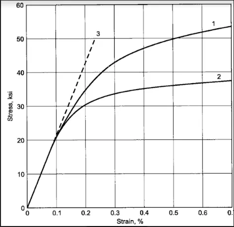
1)Power Law (MAT_018): In this material model the elasto-plastic behavior is determined by the power law of hardening. It is an isotropic model with a curve pattern depending highly on the hardening coefficient value.

`sigma_y=kepsi^n`

`sigma_y`=yield stress

`k=`strength coefficient

`epsi=`total strain

`n=`hardening coefficient

2)Piecewise linear plastic (MAT_024):

It is a material model for elasto-plastic behavior which is also an isotropic material where arbitrary stress as a function of strain curve and arbitrary strain rate dependency can be defined. The stress-strain behavior may be treated by a bilinear stress-strain curve by defining the tangent modulus, ETAN.

PROCEDURE:

Using curve 1 for Data extraction

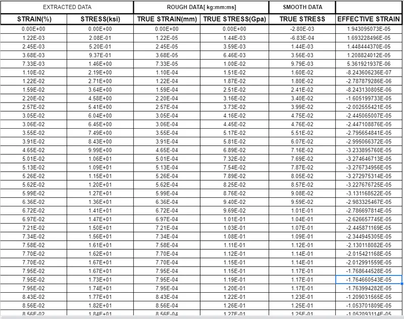
1)Extract Data using DATA DIGITIZER and unit conversion to [kg, mm, ms]

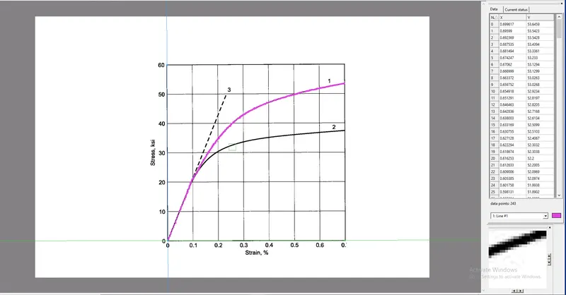
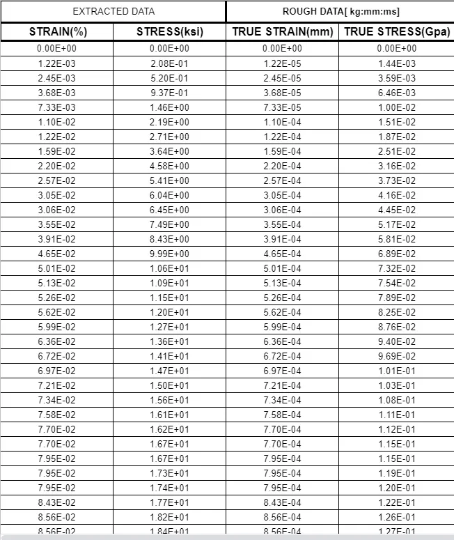
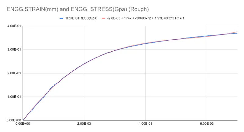
2) Smoothen the data by fitting the curve and extracting smooth stress values.

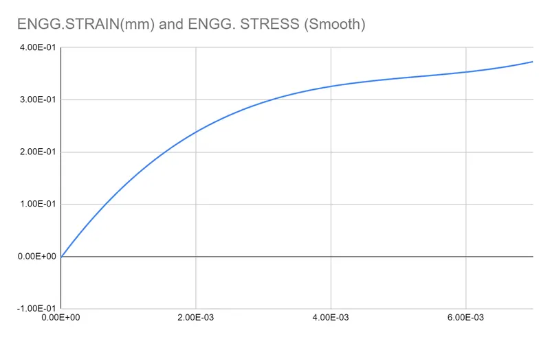
Get the best fit line from the data point using curve fitting. Then get the equation to get smooth stress values.(As shown below)

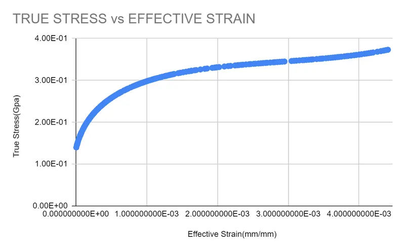
3) Processing data and create the material data required i.e true stress and effective strain value.

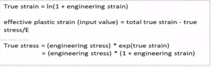
True stress and effective strain equation.

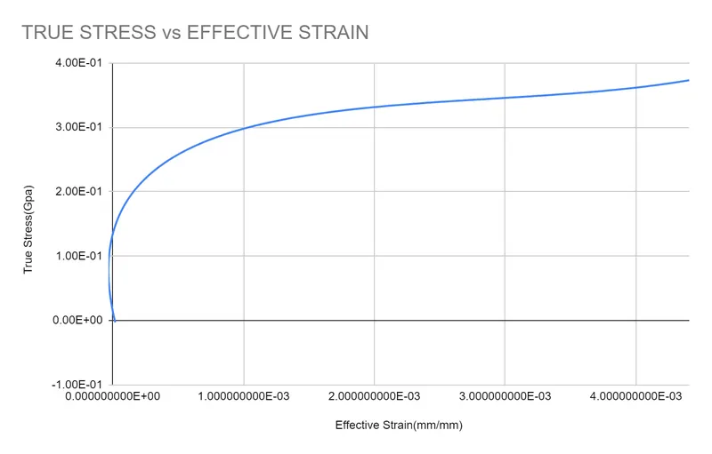
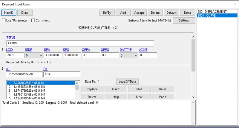
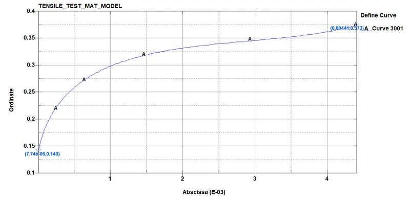
4) Define the curve in Ls-post for the material card:

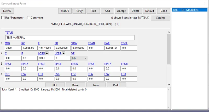
5) Define material card:

Define the LCSS ID for the curve defined by editing the card using extracted data( True stress- effective strain)

6) Define sections and part card.

The sections defined with thickness 1 mm

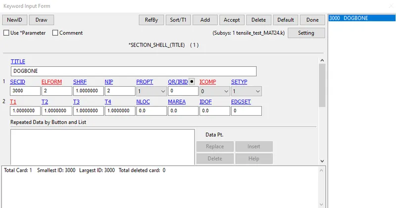
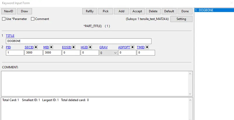
7)Define Boundary Card( prescribed motion set & SPC).

a) prescribed motion set

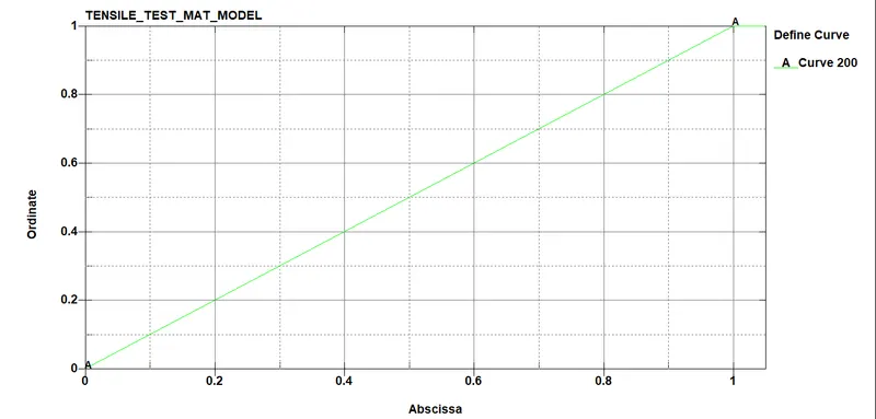
Give a displacement by defining a curve as shown below and giving S.F of 1.015mm i.e[ 145x.007= 1.015mm]

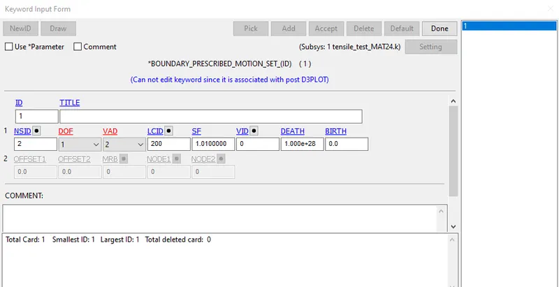
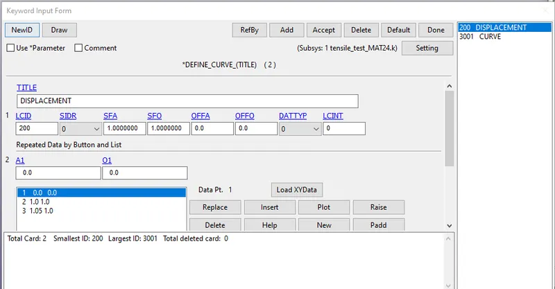
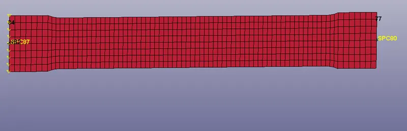
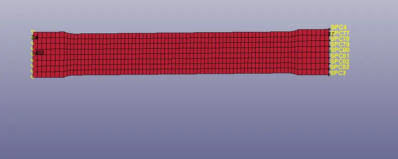
Make the node-set for the extreme left edge nodes to assign them the Prescribed Motion (displacement)

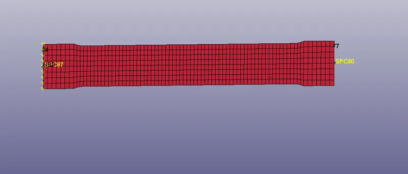
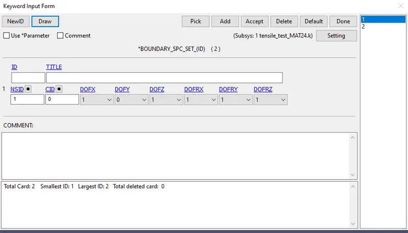
Define the SPC for the mid nodes on each side (left & right) to arrest the DOF in the Y direction (shown below)

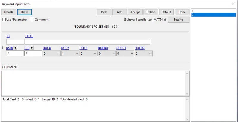
Define the SPC for the right extreme nodes on the right side to arrest the DOF in all the direction except in the Y direction (shown below)

8) Define control cards and database cards.

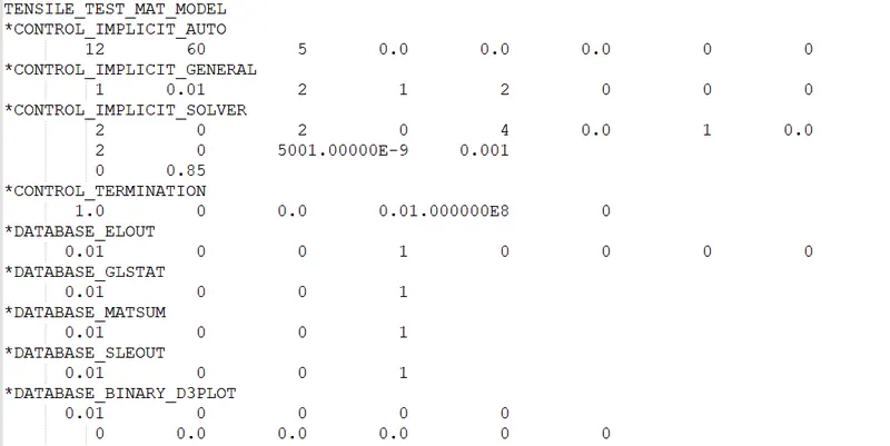
We need to define the Implicit control cards as the strain is very small and for small displacement. Therefore we have to include 3 cards i.e. implicit auto, implicit general, and implicit solver.

a)Control Cards

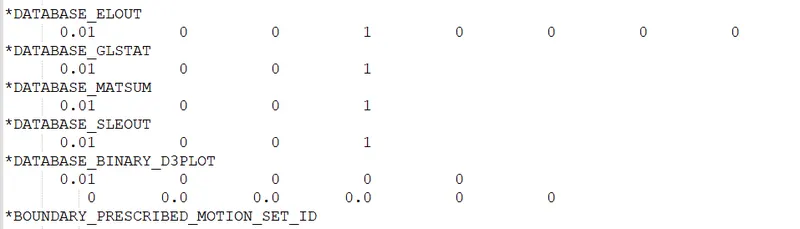
b) Database cards

RESULTS:

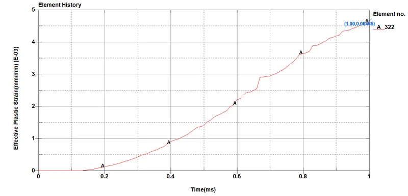
1) Effective plastic Strain plot vs time

An increasing trend w.r.t with the max value of 4.65E-03mm.

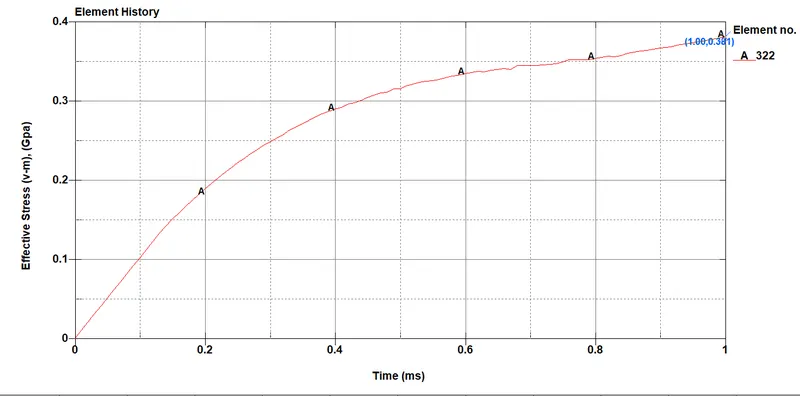
2) Effective plastic Stress plot vs time

An increasing trend w.r.t with the max value of 3.81 Gpa

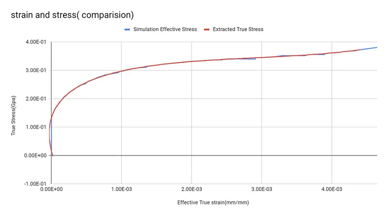
The data for stress-strain are saved and by cross plotting the data we can get the exact situation results.

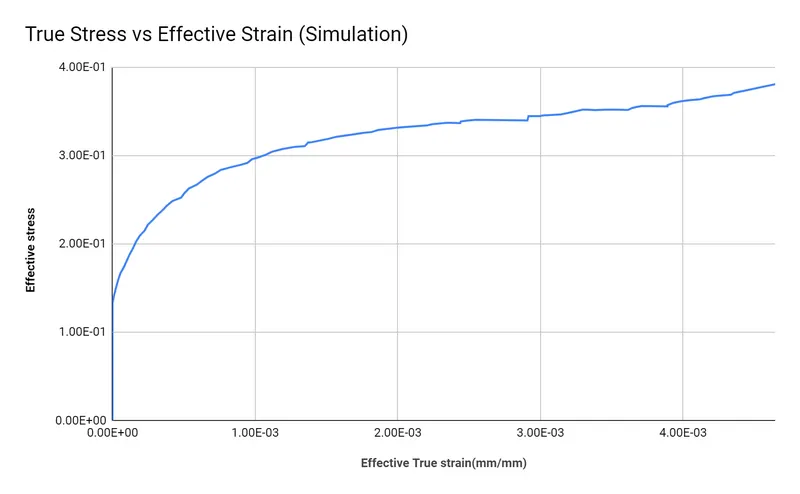
3) Cross plotting the True Stress-Effective strain(as shown below)

This is the data extracted from the diagram at the start of the assignment(shown below)

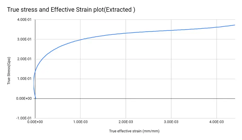
By comparing the extracted vs simulated data we can see how much the data perfectly fit the simulated curve. This validates the model which follows the extracted data from experimentation.

AREA REDUCTION

Due to elongation of the area of the dogbone reduces as shown below.

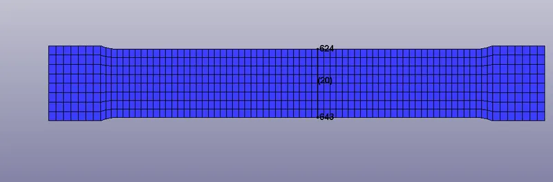
Width= 20 mm

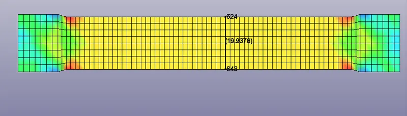
Width= 19.93 mm

ELONGATION OF LENGTH

Elongated Length = 145x (1+ .007)= 145.015mm

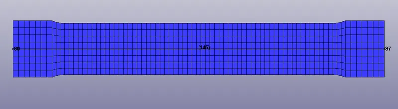
Length= 145 mm

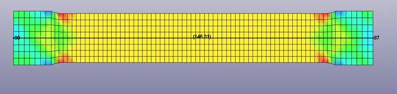
Length= 145.01 mm

Animation

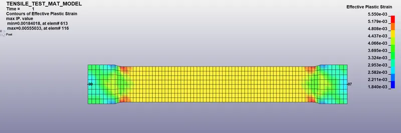
1) Von-mises Contour plot for the Effective plastic strain(at the end of simulation)

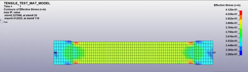
2) Von-mises Contour plot for the Effective stress(at the end of simulation)

CONCLUSION:

1. Material modeling a very important step in a CAE Analysis, this needs to be done in a careful way because wrong material data will hamper your Results.
2. Depending upon the type of data either engineering or true we need to convert them into tool compatible.
3. As this a slow process with very small deformation it is better and economical to go with an implicit approach.
4. Area reduction should be measured manually using element tool >measure.(20-19.93)* thickness=0.07*1= 0.07mm^2
5. From the stress-strain plot, we can say(visually) that 1.44 Gpa is the yield point from where the non-linear behavior starts.
6. As this is a small strain problem we can observe that the max stress and strain occurs around the fillet curved area highlighted with the red area(in the above stress-strain animation).
7. As a result, the simulated curve from LS-post fits the extracted data which validates the material model which is well satisfied.