Week - 9 Material modeling from raw data
Assignment 9
The objective of this assignment is to obtain the coordinates of several points of the stress-strain curve that are expressed in a figure. This data will be saved in a text file and then imported to LS-Dyna. A simulation will be carried in LS-Dyna and the correspondence of the results will be verified.
1. Data extraction from image
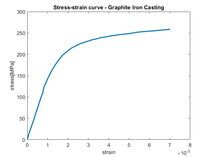
By using the software GetData Graph Digitizer, it was possible to obtain the coordinates of several points of the stress-strain curve of the material. This data was exported to a text file and then plotted in MatLab.
The stress-strain curve of the graphite iron casting is the following:
2. Young's Modulus comparison
In order to obtain the Young's Modulus, the slope of the linear section of the stress-strain curve was analysed via a finite-difference method. The resulting `\frac{d\sigma}{d\varepsilon}`curve was rather unstable (blue curve in the following image), so it was not possible to extract a Young's Modulus directly from the plot. The approach that was adopted to solve this problem was to assume the mean value of E in this section of the curve (dashed red line).
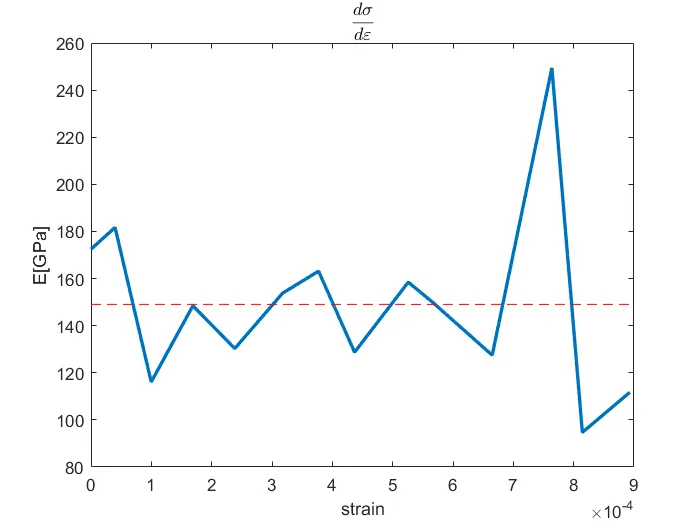
The mean value obtained for the young's modulus is `149 GPa = 21.8\times10^{6} \p\si`. Having in consideration that the standard value for the Young's Modulus of this material is `20.9\times10^{6} \p\si`, the error of this calculation is 4.31%, which seems to be acceptable.
3. Material modelling - MAT_024
MAT_024 is a elastic-plastic material model in which the young's modulus, the Poisson coefficient and the density are inputs of the material and the plasticity is defined in a piecewise linear manner.
The data retrieved from stress-strain curve will be modified to serve as an input to LS-Dyna.
The yield stress corresponds, approximately to the `\sigma_{0.2%}` value. The determination of this value is demonstrated in the following image`
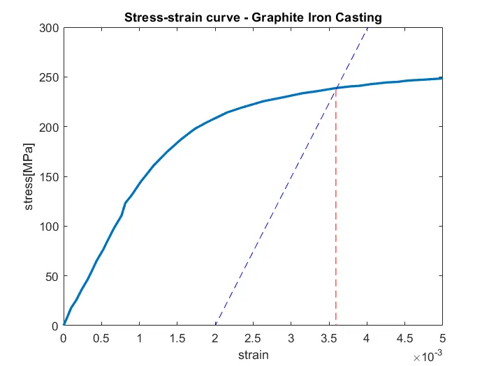
This material reaches the yield point at `\sigma = 237 MPa and \varepsilon = 0.0036`
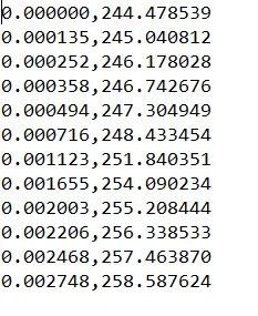
To model the plasticity zone, the following curve was imported to LS-Dyna:
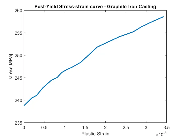
The generated text file is the following:
4. Simulation setup
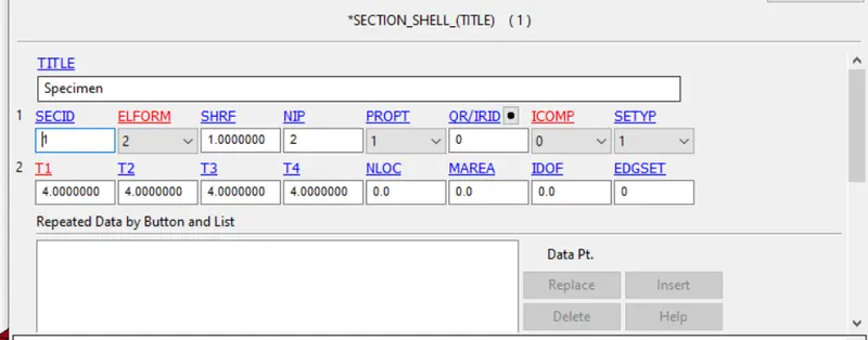
4.1. Section definition
A shell section was created with ELFORM = 2 and thickness equal to 4 mm.
4.1. Material definition
The material defined was the type MAT_024. The inputs were the following:
- Young's Modulus: E = 149 GPa
- Density:`\rho = 7.87\times10^{-6}`
- Poisson's coefficient: 0.25
4.1. Boundary conditions
4.1.1. SPC's
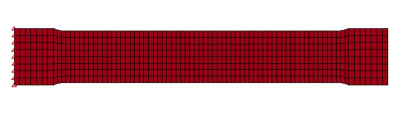
One edge of the specimen was constrained only in one DOF (along the x axis) to prevent movement in that direction. The remaining DOF's were also constrained to avoid unexpected movement. The nodes highlighted in the following image were constrained.
4.1.2. Imposed displacement
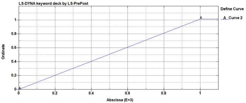
`\varepsilon = \frac{\DeltaL}{L_0} \Leftrightarrow 0.007 = \frac{\DeltaL}{145} \Leftrightarrow \DeltaL = 1.015 mm`
It was defined that the opposite edge of the specimen should displace 1.015 mm in 1000 ms (simulation time). Therefore, the curve for the imposed displacement is:
4.2. CONTROL keywords
4.2.1. CONTROL_TERMINATION
Total simulation time set to 3000 ms
4.2.2. CONTROL_ENERGY
Demand the calculation of the Hourglass energy and its inclusion in the energy balance.
4.3. DATABASE keywords
4.3.1. ASCII output
The requested outputs were MATSUM and GLSTAT
4.3.2. DATABASE_EXTENT
One of the useful results of this simulation is the plastic strain, so it is important to define this option so that the strain tensor is written in the plot file.
5. Results
The following image represents the final instant of the simulation. 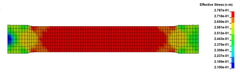
This image proves that the simulation ran as expected without unexpected movements or deformations.
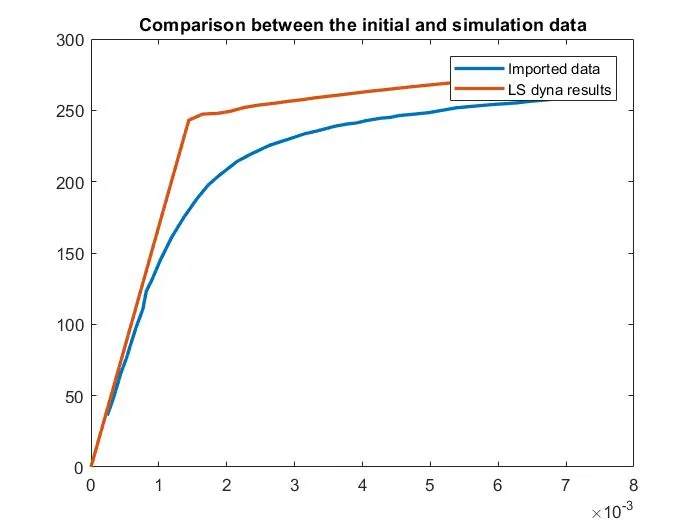
From this simulation, the maximum VonMises stress was obtained for every instant and plotted along with the strain (curve in red in the following figure). While the curve in blue corresponds to the initial data.
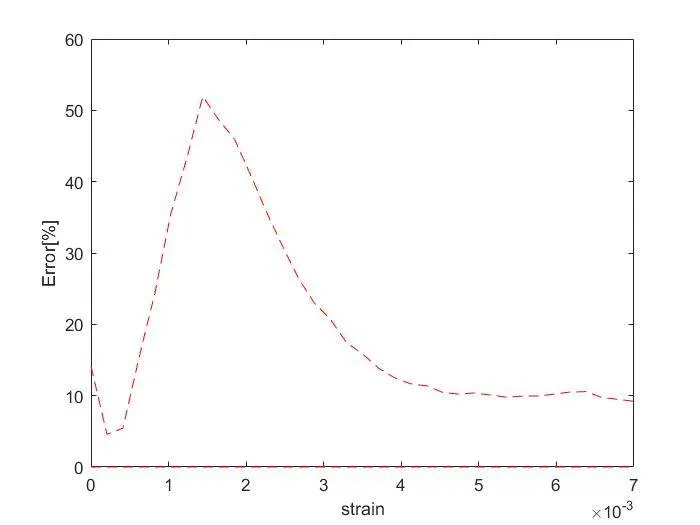
The next figure shows the relative error for each instant of the simulation.
6. Conclusion
As expected, the error is rather considerable, due to the fact that the yield stress was not determined by its exact value, but by the `\sigma_{0.2%}` value, to be later imported to the LS-Dyna model, introducing some error in the stress value. And, since the maximum strain is 0.7%, the uncertainty around the yield point is quite significant.