Week 9 - FVM Literature Review

Finite Volume Method:

The method is applied over a volume such that the governing equation is valid over the entire volume, also the properties are assumed to be concentrated at the geometric centre of the volume concerned.

Finite Difference Method:

The grid in linear and aligned so that all grids points lies in a straight line. Main thing is that the properties are considered to concentrated at a single point.

Finite Element Method:

The properties are valid over an elemental area. The properties assumed to be concentrated at area centre.

Disadvanatages of Finite Difference Method:

1. We cannot use FDM directly to a body whose grid points are not aligned properly along the x, y directions. These may occure due to complex folds, cuts in the structure.
2. As it is not aligned we cannot calculate the properties at the next adjacent point exactly, but we can some correction factor and approximate it, this method is called as 'Variable TransFormation Method' which basically seeks to create grid using different variable space which look very similar to cartesian grid.
3. Variable transformation method gives an approx solution of property but it is time consuming and complex.
4. For complex profiles, this method is less prefered.
5. That is why Finite Volume Method is used.

Interpolation Schemes in Finite Volume Method (FVM):

The interpolation schemes used in FVM method are as follows

1. Upwind Interpolation Scheme. (UDS)
2. Central Differencing Approximation. (CDS)
3. Quadratic Upwind Differencing Scheme. (QUICK)
4. Hybrid Interpolation Scheme. (CDS & UDS)
5. Total variation Diminishing Scheme. (TVD)

1. Upwind Interpolation Scheme(UDS):

In this scheme we use the node in the upwind or upstream of the given node. It is generally used for convection dominated problems (i.e Pe>1). ,

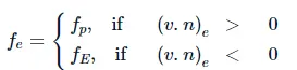
The values for this at the interface is given by

For

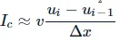(Backward differencing scheme)

For 

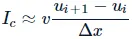(Forward differencing scheme)

 Taylor series expansion is 

where the second term has the truncation error which resembles a diffusive Flux term.

Upwind schemes are the approximations that satisfy the boundedness unconditionally and is First order accurate in space.

2.Central Differencing Approximation (CDS):

Approximate values of the variable at the control volume (CV) face centre by the linear interpolation of the values at the two nearest computational nodes.

The linear interpolation is equivalent to that of using central difference formula of the first order derivative and hence this scheme is also termed as Central Differencing Scheme(CDS).

3. Interpolation Polynomial:

The interface values are given by:

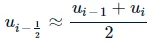and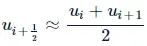

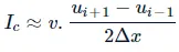(Central differencing scheme)

Taylor Series Approximation Polynomial:

The approximation is second order precise. It is the simplest and most widely used interpolation technique for the evaluation of gradients required to measure diffusive fluxes.

FLUX LIMITERS:

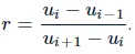
Flux limiters are used in the numerical schemes to solve problems of fluid dynamics, described by highly coupled non-linear Partial Differential Equations. If we tend to use low order numerical schemes for the solving of the governing equations then we might get a highly oscillatory and unstable solution near the discontinuity if present. Whereas if we tend to use higher-order numerical schemes to capture the phenomenon more accurately we tend to exploit the computational power unnecessarily. The main idea behind the use of the flux limiters is to limit the spatial derivative terms near the discontinuities to physical real values so as to maintain physical consistency. There are several types of flux/slope limiter functions. They come in handy when sharp wave-fronts/peaks are present. For smoothly changing waves/functions, the flux limiters do not operate and the spatial derivatives can be represented normally.

It is imperative to note that flux limiters are also referred to as slope limiters because they both have the same mathematical form, and both have the effect of limiting the solution gradient near shocks or discontinuities.

Hereflow</math>">flow = Low precision flux (1st order precise)

          fhigh</math>">fhigh= High precision flux (Highest order precision)

           ϕ(r)</math>">ϕ(r) = Flux limiter function and