Week 9 - FVM Literature Review

Aim:

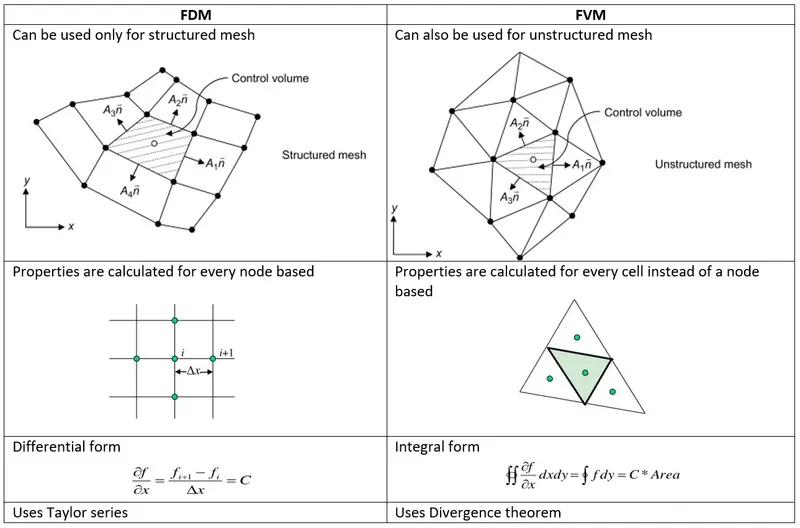
What is Finite Volume Method(FVM), write down the major differences between FDM & FVM. Also, describe the need for interpolation schemes and flux limiters in FVM. You can use the 1D linear heat conduction equation as an example.

Answer:

Finite volume method:

• In this, entire domain is divided into a finite number of cells, with small volumes.
• Cell centres act as nodes and store volume averaged of all variables.
• It is based on Guass divergence theorem, which states that integral of the divergence of the given vector over closed volume is equal to the flux of this vector across clsoed surface bonding the volume.

Difference between the FDM and FVM:

S.NO:		FINITE VOLUME METHOD (FVM)	FINITE DIFFERENCE METHOD (FDM)
1.	Grid Generation	Domain is divided into control volumes or cells with variable of interest located at the centroid of each control volume.	Domain is divided into points with each point representing variable of interest.(that are grid points)
2.	Discretization	Differential form of governing equations are integrated over each control volume i.e., discretization is based on fluxes.	Differential form of governing equations are replaced by system of algebraic equations at each grid point, or in other words, discretization is based on derivatives.
3.	Laws of conservation	Conservation principles including mass, momentum and energy are maintained by definition.	Conservation laws are not preserved in all cases.
4.	Applicability	Structured and unstructured grids as shape of control volume does not impact conservation principles.	Structured grids in most cases.
5.	Examples of Numerical Schemes	Upwind Differencing, Hybrid Differencing, Power Law : Convection-Diffusion problems	Forward difference, backward difference, central difference
6.	Advantages	Robust in terms of performance with respect to challenging problems that cover both academia and industrial physical processes, cheap in regards to quick and reliable coding.	Easier implementation, availability of higher order schemes, and generally lower computational cost and improved efficiency over FVM for problems of similar nature with simpler grid structures.
7.	Disadvantages	Presence of false diffusion when lower order accuracy upwind schemes are preferred due to stability issues in higher order accurate schemes like central differencing, and difficulty to accomplish higher order schemes in comparison to FDM.	Use of mapping functions in methods like variable transformation technique is required when point(s) are not aligned along cartesian coordinates which becomes increasingly challenging with more complex geometrical features.
8.	Applications	Physical Problems: Evaluation of external aerodynamics features of aircraft bodies, analysis of different heat transfer modes and mechanisms when graphics processing unit (GPU) on a graphics card dissipates power within an enclosed domain, assessment of wells in petroleum engineering. Commercial Softwares: ANSYS CFX, ANSYS FLUENT, PHOENICS, STAR-CD, OpenFOAM	Physical Problems: Prediction of quantities based on models developed to study weather and its attributes, astrophysics applications, seismology. Commercial Softwares: No known commercially available software, although research codes have been developed for select physical problems.

Interpolatoin schemes and flux limiters in FVM:

Interpolation schemes are used to evaluate the faces values that rise apart as convective flux and diffusive flux terms in discretization of Navier stokes equation in integral form.

1. Upwind Interpolation scheme.

• It is first order accurate interpolation scheme, bounded and has diffusive character.
• Face value is considered as cell centroid of the neighbouring cell in upwind direction.

2. Linear interpolation or central difference scheme.

• It is second order accurate interpolation scheme, unbounded and might generate oscillatory solutions.
• Face values are calculated from neighbour or owner cells.

3. Linear upwind differencing.

• It is second order accurate interpolation scheme, unbounded.
• It is used mainly for strong gradient flows.

4. Quadric upwind interpolation scheme.

• It is third order accurate interpolation scheme, high oscillatory
• Face values are approximated by three-point quadratic function.with two surrounding nodes and one upstream node.
• Flux limiters:
• These are used for second and higher order interpolations. The values are simulated using cell centroids.
• Adding a flux limiter on higher order schemes to first order schemes prevent the formation of new local maxima/minima, these are called as Total variation diminishing scheme.
• Flux limiters are also called as slope limiters, because they have same mathematical form.

1D linear heat conduction equation:

1. n = 20 plot

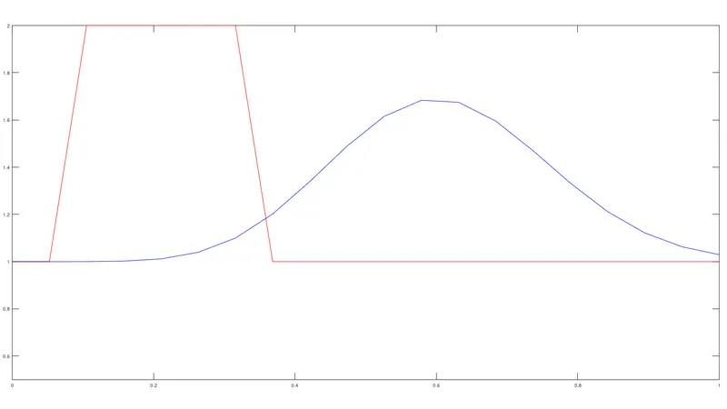
This is a velocity v/s length graph we can see that there is a drastic decrease in velocity profile. The amplitude of velocity keeps decreasing with lenght.

2. n = 40

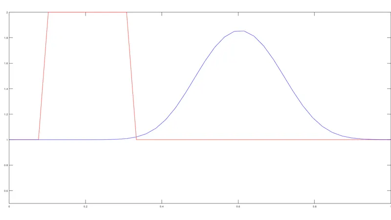
Here , there is a significant decrease in velocity profile. The truncated part is little compared to the previous graph. The amplitude of the velocity profile keeps decresing with length.

3. n = 80

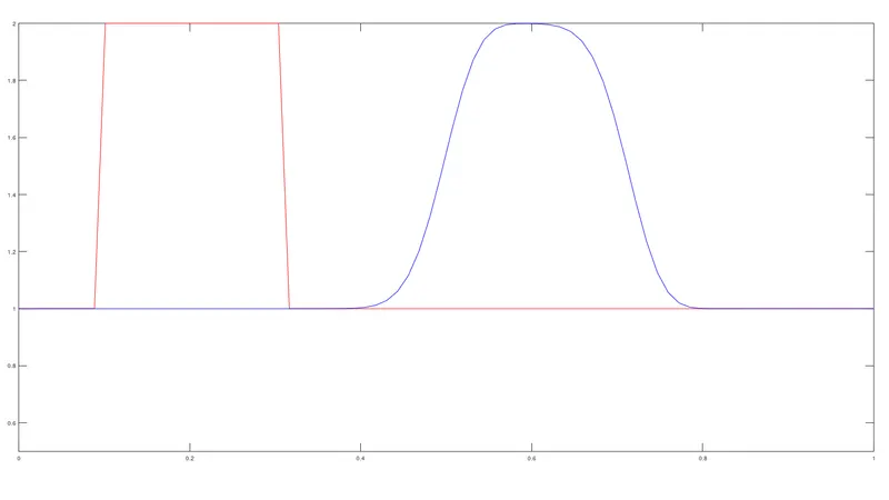
Here, there is a gradual decrease in velocity profile . The amplitude here is almost constant.

4. n = 160

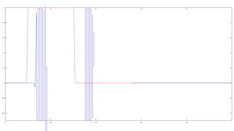
There is a disturbance in velocity profile by observing the blow up and the ripples that are formed making the graph unstable.

Comparision of the effect of time step on numerical solution

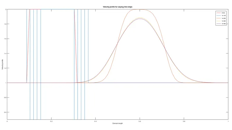
We can see that the first time step is blowing out implying that the solution is ustable . To correct this the time step value has to be corrected or within the vuable range of the solution. This can be determined by CFL condition. It is a necessary condition for convergence while solving certain PDE's.