Week 9 - FVM Literature Review

Finite Volume Method literature Review

What is Discretization?

• Discretization is the method of approximating the differential equations by a system of algebraic equations for the variables at some set of discrete locations in space and time.
• The discrete locations are grid/mesh points or cells
• The continuous information from the exact solution of PDE’s is replaced with discrete value.

Solving the PDE’s

• There are a number of methods for the solution of the governing PDE’s on the discretized domain
• The most important discretization method is:
• Finite Difference Method ( FDM)
• Finite Volume Method (FVM)
• Finite Element Method (FEM)

Finite Difference Method

• It discretized the one-dimensional convection/diffusion equation
• The derivatives were determined from a Taylor series expansion
• Simple and effective on a structured grid
• Disadvantages of FDM – conservation is not enforced unless with special treatment, restricted to simple geometries

Finite Volume Method

• Using the Finite Volume Method, the solution domain is subdivided into a finite number of small control volumes by a grid
• The grid defines to boundaries of the control volumes while the computational node lies at the center of the control volume.
• The advantage of FVM is that the integral conservation is satisfied exactly over the control volume.

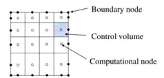
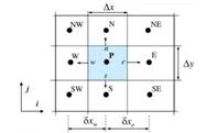
• The net flux through the control volume boundary is the sum of integrals over the four control volume faces (six in 3D). The control volumes do not overlap.
• The value of the integrand is not available at the control volume faces and is determined by interpolation.

The use of interpolation schemes to approximate the property values located at the boundaries of the control volumes are necessary when FVM is applied, using as interpolation nodes the correspondent properties located at the center of the adjacent control volumes is calculated.

We can approximate the value of the variable at CV face center by linear interpolation of the value at two nearest computational nodes. The variable e value is calculated as

`f_e = f_E lambda_e + f_p(1-lambda_e)`

`lambda_e = (X_e -X_p)/(X_E-X_P`

Flux limiter

Flux limiters are used in numerical schemes used to solve problems in fluid dynamics described by partial differential equations (PDE's). They are used in high-resolution schemes to avoid the spurious oscillations (wiggles) that arise with the high order spatial discretization schemes due to shocks, discontinuities, or sharp changes in the solution domain. The use of flux limiters, together with an appropriate high-resolution scheme, makes the solution total variation diminishing (TVD).

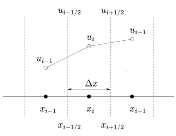
Where `F(u_(i+1/2)) and F(u_(i+1/2))`represent edge fluxes for the ith cell. If these edge fluxes can be represented by low and high resolution schemes, then a flux limiter can switch between these schemes depending upon the gradients close to the particular cell, as follows.

`F_(u_i+1/2) =f_(i+1/2)^(low) - phi(r_i)(f_(i+1/2)^(low) -f_(i+1/2)^(high) )`

`F_(u_i-1/2) =f_(i-1/2)^(low) - phi(r_i-1)(f_(i-1/2)^(low) -f_(i-1/2)^(high) )`

where `f^(low)`= low resolution flux and `f^(high)`= high resolution flux,

`phi(r)`= flux limiter function, where 'r' represents the ratio of successive gradients on the solution mesh,i.e.

`r_i = (u_i - u_(i-1))/(u_(i+1) - u_i`

The limiter function is constrained to be greater than or equal to zero, i.e., `phi(r) >= 0`